A Hierarchical Gaussian Process Model for Longitudinal Tumour Growth
We have longitudinal tumour size measurements for 10 patients. Each patient has one set of observations over about 100 days, 20 time points, recorded as the total tumour volume. We want to capture a population-level trend about how tumour size changes over time across all patients, while also allowing for patient-specific deviations from that trend.
We want to do this while properly handling uncertainty, sharing information between patients, and avoiding assumptions about parametric tumour growth curves.
Why Not a Mechanistic Two-Compartment Model?
Mechanistic models of tumour growth and shrinkage often use systems of ordinary differential equations, such as two-compartment models with proliferating and dying cells. I have explained two-compartment models in detail in here and their State-Space Bayesian inference and simulation here. These models are attractive because their parameters have biological meanings and once their parameters are estimated, they can be used to make predictions about future tumour dynamics.
However, they also have limitations:
- They impose strong assumptions about the shape of the tumour trajectory. For instance, the two-compartment model assumes a specific U-shaped form of decay and growth, which may not fit all patients well.
- They often require estimation of patient-level shrinkage, growth parameters as well as initial fractions, that may not be identifiable from sparse clinical data.
- They are less flexible in capturing patient-specific or local wiggliness.
A hierarchical Gaussian process offers a different trade-off:
- It is flexible and data-driven, having no assumptions about the shape of the tumour trajectory (the exception would be the choice of specialised kernels).
- It naturally shares information between patients.
- If kernel parameters are shared across patients, it can borrow statistical strength to improve inference for patients with sparse data.
The cost is that the inferred hyperparameters, such as lengthscales and variances, are less directly interpretable than mechanistic rate constants. And a GP model may not extrapolate well outside the observed time range, where the prediction will revert to the prior mean (zero in most cases as kernels often choose mean zero).
Model structure
Let \(y_i(t)\) be the log tumour volume for patient \(i\) at time \(t\). We model the likelihood of the observations as:
\[ y_i(t) = m(t) + g_i(t) + \varepsilon_i(t) \]
where:
- \(m(t)\) is a population-level mean function, capturing a shared trend (latent curve) that all patients follow. It describes the correlations between observations from any patients and at any times (“any-to-any” correlation).
- \(g_i(t)\) is a patient-specific deviation. Therefore, the correlation bewteen two observations from the same patient is defined by both \(m(t)\) and \(g_i(t)\), while the correlation between two observations from different patients is defined only by \(m(t)\).
- \(\varepsilon_i(t) \sim \mathcal{N}(0, \sigma_n^2)\) is measurement noise, local to each observation and independent across patients and time.
- Adding measurement noise to likelihood is mathematically equivalent to adding \(\sigma_n^2\) to the diagonal of the covariance matrix of the GP prior of \(g_i(t)\).
We place Gaussian process priors on \(m\) and \(g_i\):
\[ m(t) \sim \mathcal{GP}(0, k_m) \]
\[ g_i(t) \sim \mathcal{GP}(0, k_g+\sigma_n^2 I) \]
Both \(m\) and \(g_i\) have zero mean functions. The kernels \(k_m\) and \(k_g\) capture smoothness and amplitude.
Kernel Choices
For both population and patient-specific GPs, we use radial basis function (RBF) kernels, also known as squared exponential kernels. These kernels are infinitely differentiable and produce very smooth functions. We use different hyperparameters for the population and patient-specific kernels, allowing the patient deviations to be more flexible than the population mean, by placing a shorter lengthscale prior on the patient deviations.
For simplicity, we do not set hierachical priors on the kernel hyperparameters, but this is a natural extension if we have many patients and want to allow for patient-specific lengthscales or amplitudes.
\[ k_{m,g}(t, t') = \sigma_{m,g}^2 \exp\left(-\frac{(t - t')^2}{2\ell_{m,g}^2}\right) \]
There are in total four hyperparameters: \(\ell_m, \ell_g, \sigma_m, \sigma_g\) for the two kernels, plus \(\sigma_n\) for the noise standard deviation.
Priors on Hyperparameters
We place weakly informative priors on the kernel hyperparameters to avoid extreme values.
For lengthscales, we need positive real values. As the time is recorded in days and our existing knowledge says that tumours shrink for about 4 weeks before drug resistance starts. For a GP with an RBF kernel to produce such a shape, the lengthscale must be short enough for the curve to bend noticeably within the observed time window. If the lengthscale is much larger than the time range, the GP cannot produce a dip and rise — it will look flat or monotonic.
We may also choose to scale the time to have mean zero and standard deviation one (at each patient level or globally). In this case, we expect the lengthscales to be of order one. Values less than one have functions wiggle faster than the sampling rate, whereas larger than one means the function is essentially flat. Hence, we want a prior distribution concentrated around one, but penalise extreme small or large values. We also want a prior that is scale-invariant, so that when we change scale in the future, the prior still makes sense. Therefore, log-nomral is a better choice than inverse-gamma, because scalling \(\ell\) by a constant factor (\(c\)) will just shift the mean of the log-normal distribution by \(\log(c)\), preserving the shape of the prior. Scaling the time will make it easier to set priors for lengthscale. However, time need to be scaled back for posterior predictives.
\[ \log \ell \sim \mathcal{N}(\mu_\ell, \sigma_\ell^2) \]
For population lengthscale, we choose a slightly wider prior because population trend tends to be smoother than patient deviations. And the mean is on log-scale, therefore the real mean is \(e^{\mu_{\ell_m}}=25\). We set:
\[ \mu_{\ell_m} = \log(25), \quad \sigma_{\ell_m} = 0.25 \]
For patient-specific lengthscale, we delibarately choose a smaller mean (\(e^{\mu_{\ell_g}} = 20\)) to encourage shorter lengthscales, which allows patient deviations to be more flexible:
\[ \mu_{\ell_g} = \log(20), \quad \sigma_{\ell_g} = 0.25 \]
For amplitudes, we also need positive values, and we prefer small variation unless data demands otherwise. We use half-normal distributions to have the mass near zero but allow for larger values:
\[ \sigma_{m,g} \sim \mathcal{N}^+(0, 0.1) \]
For the noise standard deviation, we also use a half-normal prior, with larger variance to encourage potentially more noise:
\[ \sigma_n \sim \mathcal{N}^+(0, 1) \]
These are weak enough to let the data dominate while keeping the model well-behaved.
Data Transformation
Tumour volume is positive and typically right-skewed. We therefore model log volume:
\[ y_i^{\log} = \log(\text{observed\_total} + 1\mathrm{e}{-6}) \]
We then standardise the log volume and time so that the GP priors are centred around zero. This helps with setting up priors, sampling and interpretation.
\[ y_i^{\text{std}} = \frac{y_i^{\log} - \bar{y}^{\log}}{s_{y^{\log}}} \]
where \(\bar{y}^{\log}\) is the mean of all log volumes across all patients and times, and \(s_{y^{\log}}\) is the standard deviation.
This transformation centres the data around zero and scales it to unit variance. It helps the GP prior (which has zero mean) match the data, and it improves sampling efficiency.
After fitting, we can transform it back for plotting and interpretation:
\[ y_i^{\log} = y_i^{\text{std}} \cdot s_{y^{\log}} + \bar{y}^{\log} \]
We can standardise time, although standardisation is not chosen this time:
\[ t_i^{\text{std}} = \frac{t_i - \bar{t}}{s_t} \]
where \(\bar{t}\) is the mean of all time points (or time points per patient) and \(s_t\) is the corresponding standard deviation.
This transformation, although make lengthscale difficult to interpret, can increase numerical stability. After fitting, we should always transform the time back:
\[ t_i = t_i^{\text{std}} \cdot s_t + \bar{t} \]
Stan Code
Below is a Stan implementation using the marginal likelihood form. We integrate out the latent Gaussian processes (\(m(t), g_i(t)\)) by directly setting up the combined covariance matrix:
\[ K_{i,j} = k_m(t_i, t_j) + \begin{cases} k_g(t_i, t_j) + \sigma_n^2 \delta_{i, j} & \text{if } id_i = id_j \\ 0 & \text{if } id_i \neq id_j \end{cases} \]
This is exactly what the Stan code builds:
- i and j index all observations across all patients.
- The loop over \(i, j\) adds \(k_m(t_i, t_j)\) for every pair, regardless of patient.
- It adds \(k_g(t_i, t_j)\) only when \(id_i = id_j\) (meaning when two observations come from the same patient).
- \(\delta_{i, j}\) is the Kronecker delta, which is 1 if \(i = j\) and 0 otherwise. In practice, we add \(\sigma_n^2\) to the diagonal of the covariance matrix. Intuitively, this means that the noise is independent across observations, so it only contributes to the variance of each observation (same patient at same time), not the covariance between different observations.
The resulting matrix has a nested block structure:
- Outer blocks correspond to patients; Inner blocks correspond to time points within each patient or cross-patients.
- Within a patient block (the diagonal of the outer blocks): entries are \(k_m + k_g\) (off-diagonal) or \(\sigma_m^2 + \sigma_g^2 + \sigma_n^2\) (diagonal, because these are same time points, so \(k=\sigma^2\exp(0)\)).
- Cross patient blocks (off-diagonal of the outer blocks): entries are \(k_m\) only.
For example, for two patients, each with two time points:
\[ K = \begin{bmatrix} \underbrace{\begin{matrix} \sigma_m^2 + \sigma_g^2 + \sigma_n^2 & k_m(t_1,t_2) + k_g(t_1,t_2) \\ k_m(t_2,t_1) + k_g(t_2,t_1) & \sigma_m^2 + \sigma_g^2 + \sigma_n^2 \end{matrix}}_{\text{Patient 1 block}} & \underbrace{\begin{matrix} k_m(t_1,t_1) & k_m(t_1,t_2) \\ k_m(t_2,t_1) & k_m(t_2,t_2) \end{matrix}}_{\text{cross-patient block}} \\ \underbrace{\begin{matrix} k_m(t_1,t_1) & k_m(t_1,t_2) \\ k_m(t_2,t_1) & k_m(t_2,t_2) \end{matrix}}_{\text{cross-patient block}} & \underbrace{\begin{matrix} \sigma_m^2 + \sigma_g^2 + \sigma_n^2 & k_m(t_1,t_2) + k_g(t_1,t_2) \\ k_m(t_2,t_1) + k_g(t_2,t_1) & \sigma_m^2 + \sigma_g^2 + \sigma_n^2 \end{matrix}}_{\text{Patient 2 block}} \end{bmatrix} \]
Unfold to see the Stan code for this hierarchical GP model
data {
  int<lower=1> N;                    // total number of observations
  int<lower=1> P;                    // number of patients
  array[N] int<lower=1,upper=P> id;  // patient id for each observation
  vector[N] t;                       // standardised time
  vector[N] y;                       // standardised log volume
}

parameters {
  // declare hyperparameters to be more than zero
  real<lower=0> length_m;
  real<lower=0> length_g;
  real<lower=0> sigma_m;
  real<lower=0> sigma_g;
  real<lower=0> sigma_n;
}

model {
  // Priors for scaled time
  //log(length_m) ~ normal(0, 1.5);
  //log(length_g) ~ normal(-0.5, 1);
  // Lengthscale priors on original time scale
  log(length_m) ~ normal(log(25), 0.25);  // population mean, ~25 days
  log(length_g) ~ normal(log(20), 0.25);  // patient deviation, ~20 days
  // following will be automatically truncated to be positive due to <lower=0> constraint
  sigma_m ~ normal(0, 0.1);
  sigma_g ~ normal(0, 0.1);
  sigma_n ~ normal(0, 1);

  // Marginal likelihood: y ~ N(0, K)
  // K has block structure with population and patient-specific components.
  // We construct it using Cholesky factor in transformed parameters or use
  // a custom multi-normal with covariance depending on id.

  // For efficiency, use a loop over patients and build the full covariance.
  // This is straightforward but can be optimised.
  matrix[N, N] K;

  for (i in 1:N) {
    for (j in i:N) {
      real k_m = sigma_m^2 * exp(-0.5 * square((t[i] - t[j]) / length_m));
      real k_g = 0.0;
      if (id[i] == id[j]) {
        k_g = sigma_g^2 * exp(-0.5 * square((t[i] - t[j]) / length_g));
      }
      K[i, j] = k_m + k_g;
      K[j, i] = k_m + k_g;
    }
    K[i, i] += sigma_n^2;
  }

  y ~ multi_normal(rep_vector(0, N), K);
}
Scaling Up: Marginal Likelihood with a Low-Rank Population Mean
The Stan model above builds the full \(N \times N\) covariance matrix, where \(N\) is the total number of observations. Every entry of this matrix depends on the population kernel \(k_m\), which creates correlations between all observations, including across different patients. Although it is a clear way to show how covariance matrix is constructed, inverting this matrix costs \(O(N^3)\), which becomes slow for even moderate datasets.
What is \(O(N^3)\)?
This is Big-O notation, which describes how the computational cost of an algorithm grows as the input size grows. If you have a matrix of size \(N \times N\), the cost of inverting it or computing its Cholesky decomposition grows proportionally to \(N^3\).
For example:
- \(N = 100\): cost is proportional to \(100^3 = 1{,}000{,}000\)
- \(N = 1000\): cost is proportional to \(1000^3 = 1{,}000{,}000{,}000\)
Doubling \(N\) increases the cost by a factor of 8. This is why large GP models become slow very quickly.
How to Construct \(\Phi\)
Let \(Z = \{z_1, \dots, z_M\}\) be a set of inducing points, typically chosen as a grid over the time range. Let \(K_{ZZ}\) be the \(M \times M\) population covariance at these inducing points, and let \(K_{XZ}\) be the \(N \times M\) cross-covariance between observations and inducing points. Then:
\[ \Phi = K_{XZ} L_{ZZ}^{-\top} \]
where \(L_{ZZ}\) is the Cholesky factor of \(K_{ZZ}\), so that \(K_{ZZ} = L_{ZZ} L_{ZZ}^\top\). And \(-\top\) means inverse the matrix before transposing it. This construction guarantees that:
\[ \Phi \Phi^\top = K_{XZ} K_{ZZ}^{-1} K_{ZX} \approx K_m \]
Because: \[ \Phi \Phi^\top = K_{XZ} L_{ZZ}^{-\top} \left( K_{XZ} L_{ZZ}^{-\top} \right)^\top = K_{XZ} L_{ZZ}^{-\top} L_{ZZ}^{-1} K_{ZX} = K_{XZ} (L_{ZZ} L_{ZZ}^\top)^{-1} K_{ZX} = K_{XZ} K_{ZZ}^{-1} K_{ZX} \]
This is the Nyström approximation of the population covariance.
What is the Cholesky factor?
For a symmetric positive definite matrix \(K\), the Cholesky decomposition is:
\[ K = L L^\top \]
where \(L\) is a lower triangular matrix with positive diagonal entries. This is analogous to the scalar square root: \(K = L L^\top\) is like \(k = \sqrt{k} \cdot \sqrt{k}\).
We apply the Cholesky decomposition to \(K_{ZZ}\), the covariance at the inducing points. It gives \(K_{ZZ} = L_{ZZ} L_{ZZ}^\top\).
Why \(K_{ZZ}^{-1}\) is needed in Nyström approximation?
Let \(K_{XZ}\) be \(N \times M\) and \(K_{ZX}\) be \(M \times N\). Their product is:
\[ (K_{XZ} K_{ZX})_{ij} = \sum_{m=1}^{M} [K_{XZ}]_{im} [K_{ZX}]_{mj} \] where:
- \([K_{XZ}]_{im} = k(t_i, z_m)\)
- \([K_{ZX}]_{mj} = k(z_m, t_j)\)Therefore: \[ (K_{XZ} K_{ZX})_{ij} = \sum_{m=1}^{M} k(t_i, z_m) \, k(z_m, t_j) \] This is a sum of products of kernel values, which is not the same as evaluating the kernel directly at \(t_i\) and \(t_j\), because the kernel is not generally a sum of products of its values at intermediate points. The true population covariance is:
\[ [K_m]_{ij} = k(t_i, t_j) \]
The matrix \(K_{ZZ}^{-1}\) acts as a correction. It ensures that the approximation reproduces the kernel as accurately as possible given only the inducing points.
Intuitively:
- \(K_{XZ}\) tells you how each observation relates to the inducing points.
- \(K_{ZX}\) tells you how the inducing points relate to each observation.
- Without \(K_{ZZ}^{-1}\), you are effectively double-counting the inducing point information.
- With \(K_{ZZ}^{-1}\), you correctly weight the inducing point contributions so that the result matches the true kernel when the function is in the span of the inducing point basis.
The Marginal Likelihood based on inducing points
In the marginal likelihood formulation, we do not sample the latent functions \(m(t)\) and \(g_i(t)\) explicitly. We integrate them out, which leaves us with a Gaussian distribution for the observed data:
\[ \mathbf{y} \sim \mathcal{N}(\mathbf{0}, K) \]
where \(K = B + \Phi \Phi^\top\) is the covariance of the observations.
The quantity Stan needs is the likelihood \(p(\mathbf{y} \mid \theta)\), which is the probability density of this multivariate Gaussian, viewed as a function of the hyperparameters \(\theta\). In the GP literature, this is often called the marginal likelihood because the latent functions have been marginalised out.
\[ p(\mathbf{y}) = \frac{1}{(2\pi)^{N/2} \det(K)^{1/2}} \exp\left(-\frac{1}{2}\mathbf{y}^\top K^{-1} \mathbf{y}\right) \]
To evaluate it, we need two ingredients from the multivariate Gaussian density:
- The inverse \(K^{-1}\), which appears in the quadratic form \(\mathbf{y}^\top K^{-1} \mathbf{y}\).
- The determinant \(\det(K)\), which appears in the normalising constant.
Because \(B\) is block diagonal and \(\Phi \Phi^\top\) is low rank, we can use the Woodbury identity (full formula see here) to compute the marginal likelihood without inverting the full \(N \times N\) matrix:
\[ (B + \Phi \Phi^\top)^{-1} = B^{-1} - B^{-1} \Phi \left( I_M + \Phi^\top B^{-1} \Phi \right)^{-1} \Phi^\top B^{-1} \]
The determinant is:
\[ \det(B + \Phi \Phi^\top) = \det(B) \det\left( I_M + \Phi^\top B^{-1} \Phi \right) \]
The key computational advantages:
- \(B^{-1}\) is cheap because \(B\) is block diagonal by patient. Each patient block has size \(n_i \times n_i\) (n_i is the time points for a specific patient), so inversion costs \(O(\sum_i n_i^3)\), which is much less than \(O(N^3)\).
- \(\Phi^\top (B^{-1} \Phi)\) results in multiplying \(M \times N\) by \(N \times M\). Each entry of the result requires \(N\) multiplications, and there are \(M^2\) entries. It costs \(O(N M^2)\). Inversing this \(M \times M\) matrix costs \(O(M^3)\).
- \(B^{-1} \Phi\) costs \(\sum_i n_i^2 M\).
- Multiply \(B^{-1} \Phi\) by the \(M \times M\) inverse: cost \(O(N M^2)\).
- Multiply the result by \(\Phi^\top B^{-1}\): cost \(O(N M^2)\).
- The overall dominant cost is \(O(N M^2 + \sum_i n_i^3)\), which scales linearly in \(N\) for fixed \(M\).
- Intuitively, we are saying the cost of inverting the low-rank population mean matrix is the cost of multiplying the low-rank factor \(\Phi\) (size \(N \times M\)) with other matrices. It grows linearly with \(N\) and quadratically with \(M\).
This is the standard sparse GP approximation, adapted to the hierarchical structure.
Updated Stan Code
Below is the updated Stan model. The key changes:
- The population mean \(m(t)\) is now approximated using \(M\) inducing points.
- The covariance for \(m\) is constructed from the inducing points and added as a low-rank component.
- The patient-specific covariance and noise remain block diagonal.
Briefly, the Stan code models observations following the log-density of the multivariate Gaussian, and we can ignore the normalising constant \(-\frac{N}{2}\log(2\pi)\):
\[ \log p(\mathbf{y}) = -\frac{N}{2}\log(2\pi) - \frac{1}{2}\log\det(K) - \frac{1}{2}\mathbf{y}^\top K^{-1} \mathbf{y} \]
Using the Woodbury identity, we can express both the determinant and the inverse of \(K = B + \Phi\Phi^\top\) in terms of cheap quantities. \[ \log\det(K) = \log\det(B) + \log\det\left(I_M + \Phi^\top B^{-1} \Phi\right) \]
In the code:
- \(\log\det(B)\) is log_det_B
- \(\log\det(I_M + \Phi^\top B^{-1} \Phi)\) is log_det_middle
- middle \(= I_M + \Phi^\top B^{-1} \Phi\)
\[ K^{-1} = B^{-1} - B^{-1} \Phi \left(I_M + \Phi^\top B^{-1} \Phi\right)^{-1} \Phi^\top B^{-1} \]
The quadratic form \(\mathbf{y}^\top K^{-1} \mathbf{y}\) then becomes:
\[ \mathbf{y}^\top K^{-1} \mathbf{y} = \mathbf{y}^\top B^{-1} \mathbf{y} - \mathbf{y}^\top B^{-1} \Phi \left(I_M + \Phi^\top B^{-1} \Phi\right)^{-1} \Phi^\top B^{-1} \mathbf{y} \]
In the code:
- First term: dot_product(y, B_inv * y) which is \(\mathbf{y}^\top B^{-1} \mathbf{y}\) - Second term: define rhs = Phi' * (B_inv * y) which is \(\Phi^\top B^{-1} \mathbf{y}\), then compute dot_product(rhs, mdivide_left(middle, rhs)), which is \(\mathbf{r}^\top \text{middle}^{-1} \mathbf{r}\).
- The difference between the first and second term is quad.
In the model block, as we computed the Woodbury-rewritten log-density to avoid inverting the full \(N \times N\) covariance matrix during sampling, which would be very slow. Hence we use target to implement this custom likelihoods in Stan.
In the generated quantities block, we can safely use the standard multi_normal_rng because it runs only after sampling and does not affect the Markov chain, so the extra cost of a full Cholesky decomposition is acceptable.
Unfold to see the updated Stan code
data {
  int<lower=1> N;                          // total observations
  int<lower=1> P;                          // number of patients
  int<lower=1> M;                          // number of inducing points
  array[N] int<lower=1,upper=P> id;        // patient id per observation
  vector[N] t;                             // standardised time
  vector[N] y;                             // standardised log volume
  vector[M] z;                             // inducing points (standardised time)
}

parameters {
  real<lower=0> length_m;
  real<lower=0> length_g;
  real<lower=0> sigma_m;
  real<lower=0> sigma_g;
  real<lower=0> sigma_n;
}

transformed parameters {
  matrix[N, M] K_XZ;
  matrix[M, M] K_ZZ;
  matrix[M, M] L_ZZ;
  matrix[N, M] Phi;

  // Build population covariances at inducing and observation points
  // Build Phi
  for (i in 1:N) {
    for (j in 1:M) {
      K_XZ[i, j] = sigma_m^2 * exp(-0.5 * square((t[i] - z[j]) / length_m));
    }
  }
  for (i in 1:M) {
    for (j in 1:M) {
      K_ZZ[i, j] = sigma_m^2 * exp(-0.5 * square((z[i] - z[j]) / length_m));
    }
    K_ZZ[i, i] += 1e-6;   // jitter for diagonal ensure positive definiteness and stabilizes decomposation.
  }
  L_ZZ = cholesky_decompose(K_ZZ);
  Phi = K_XZ / L_ZZ'; // Phi = K_XZ * L_ZZ^{-T}

  // Build block-diagonal B (patient-specific + noise)
  // and store its inverse and log-determinant.
  // We loop over patients to build B_i, invert, and accumulate. This way is computationally more efficient than building the whole B, then invert and log_determinant
  matrix[N, N] B = rep_matrix(0, N, N);
  matrix[N, N] B_inv = rep_matrix(0, N, N);
  real log_det_B = 0;

  for (p in 1:P) {
    // indices of observations belonging to patient p
    array[N] int idx;
    int n_p = 0;
    for (i in 1:N) {
      if (id[i] == p) {
        n_p += 1;
        idx[n_p] = i; //for each patient's observation, assign it a global
      }
    }
    if (n_p > 0) {
      matrix[n_p, n_p] B_p;
      for (a in 1:n_p) {
        for (b in 1:n_p) {
          B_p[a, b] = sigma_g^2 * exp(-0.5 * square((t[idx[a]] - t[idx[b]]) / length_g));
        }
        B_p[a, a] += sigma_n^2;
      }
      // Invert B_p and place into B_inv (globally indexed matrix)
      matrix[n_p, n_p] B_p_inv = inverse(B_p);
      log_det_B += log_determinant(B_p);
      for (a in 1:n_p) {
        for (b in 1:n_p) {
          B_inv[idx[a], idx[b]] = B_p_inv[a, b];
        }
      }
    }
  }
}

model {
  // Priors
  //log(length_m) ~ normal(0, 1.5);
  //log(length_g) ~ normal(-0.5, 1);
  // Lengthscale priors in original time units
  log(length_m) ~ normal(log(25), 0.25);  // population mean, ~25 days
  log(length_g) ~ normal(log(20), 0.25);  // patient deviation, ~20 days
  // following will be automatically truncated to be positive due to <lower=0> constraint
  sigma_m ~ normal(0, 0.1);
  sigma_g ~ normal(0, 0.1);
  sigma_n ~ normal(0, 1);

  // Woodbury: compute B^{-1} Phi and the small M x M matrix
  matrix[N, M] B_inv_Phi = B_inv * Phi;
  matrix[M, M] middle = add_diag(Phi' * B_inv_Phi, 1.0);   // I_M + Phi' B^{-1} Phi

  // Log marginal likelihood
  real log_det_middle = log_determinant(middle);
  vector[M] rhs = Phi' * (B_inv * y);
  real quad = dot_product(y, B_inv * y) - dot_product(rhs, mdivide_left(middle, rhs));

  // Stan's unnormalized log posterior accumulator; target += adds custom (not standard distribution) log-density terms
  target += -0.5 * (log_det_B + log_det_middle + quad);
}

generated quantities {
  vector[N] y_rep;
  // Reconstruct the full covariance K for the observed data
  matrix[N, N] K_full = B + Phi * Phi';

  // Add small jitter to ensure positive definiteness
  for (i in 1:N) {
    K_full[i, i] += 1e-8;
  }

  // Draw a replicated dataset (posterior predictive) from the model
  y_rep = multi_normal_rng(rep_vector(0, N), K_full);
}
Infer the model in R
In R, prepare the inducing points \(z\) as a grid over the standardised time range.
The following code also include diagnostics for convergence.
We look for:
- R-hat values close to 1 (< 1.01)
- ESS > 400
- Trace plots showing good mixing
Unfold to see the R code for fitting the model
# 1. Core packages (infrastructure)
library(rstan)
library(StanHeaders)
library(cmdstanr)
# 2. Data manipulation (if needed)
library(dplyr)
library(tidyr)
# 3. Visualization (depends on ggplot2)
library(ggplot2)
library(bayesplot)  # Depends on ggplot2, loads after it
library(patchwork)
library(cowplot) # make combined plot define ncol
# 4. Other analysis packages
library(posterior)

# Load data, in our case dat, having columns: time, patient, observed_total

# Transform
dat$y_log <- log(dat$observed_total + 1e-6)

# Standardise log volume globally
y_mean <- mean(dat$y_log)
y_sd <- sd(dat$y_log)
dat$y_std <- (dat$y_log - y_mean) / y_sd

# define inducing points
M <- 10
z <- seq(min(dat$t_std), max(dat$t_std), length.out = M)

# Prepare Stan data
stan_data <- list(
  N = nrow(dat),
  P = n_distinct(dat$patient),
  M = M,
  id = as.integer(as.factor(dat$patient)),
  t = dat$time,
  y = dat$y_std,
  z=z
)

# Compile model
mod <- cmdstan_model("GP_RBF_tumourgrowth_lowrank.stan")

# Fit
fit <- mod$sample(
  data = stan_data,
  seed = 123,
  chains = 4,
  parallel_chains = 4,
  iter_warmup = 1000,
  iter_sampling = 1000
)

#### Check model convergence ####
# Print summary
summ <- fit$summary(variables = c("length_m", "length_g", "sigma_m", "sigma_g", "sigma_n"))

# Trace plots
small_draws <- fit$draws(variables = c("length_m", "length_g", "sigma_m", "sigma_g", "sigma_n"))
p_trace<-mcmc_trace(small_draws,
        pars = c("length_m", "length_g", "sigma_m", "sigma_g", "sigma_n"),
        facet_args = list(ncol = 5))+
        scale_x_continuous(breaks = seq(0, 1000, by = 500))+
        ggtitle("Trace plots")

# Posterior distributions ##
# Plot 1: length_m and length_g
p1 <- mcmc_areas(
  small_draws,
  pars = c("length_m", "length_g")
)
# Plot 2: sigma_m, sigma_g, sigma_n
p2 <- mcmc_areas(
  small_draws,
  pars = c("sigma_m", "sigma_g", "sigma_n")
)
combined<-plot_grid(p1, p2, ncol = 2,rel_widths = c(1, 1))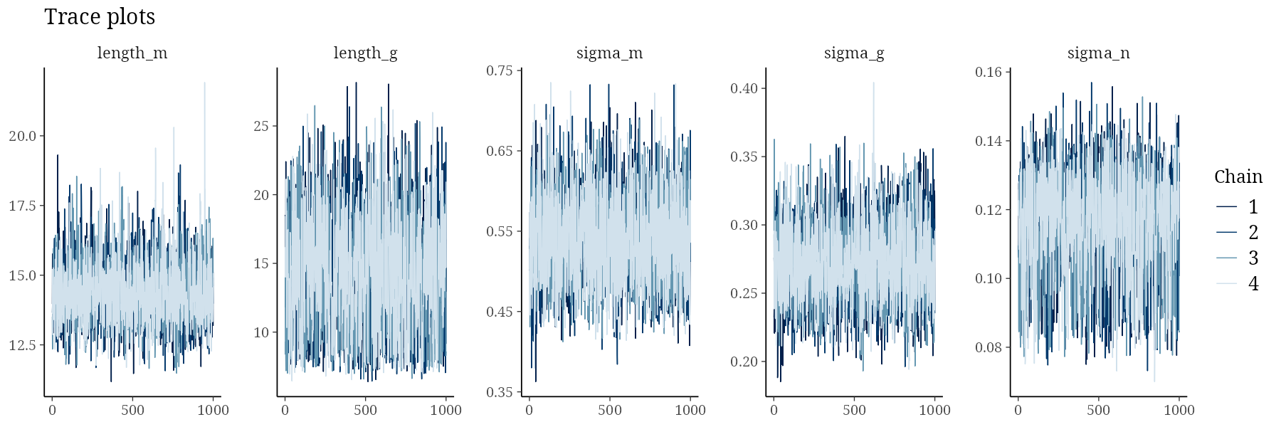
| variable | mean | median | sd | mad | q5 | q95 | rhat | ess_bulk | ess_tail |
|---|---|---|---|---|---|---|---|---|---|
| length_m | 14.44 | 14.35 | 1.12 | 1.09 | 12.80 | 16.38 | 1.00 | 2509.03 | 1739.65 |
| length_g | 14.15 | 14.14 | 4.00 | 4.34 | 8.04 | 20.86 | 1.00 | 1581.33 | 2604.05 |
| sigma_m | 0.54 | 0.54 | 0.05 | 0.05 | 0.46 | 0.63 | 1.00 | 3060.15 | 2513.11 |
| sigma_g | 0.27 | 0.27 | 0.03 | 0.03 | 0.23 | 0.32 | 1.00 | 2656.30 | 2250.94 |
| sigma_n | 0.12 | 0.12 | 0.01 | 0.01 | 0.09 | 0.14 | 1.01 | 1591.66 | 2120.46 |
Posterior Predictive Plots
Why the Default GP Does Not Fit
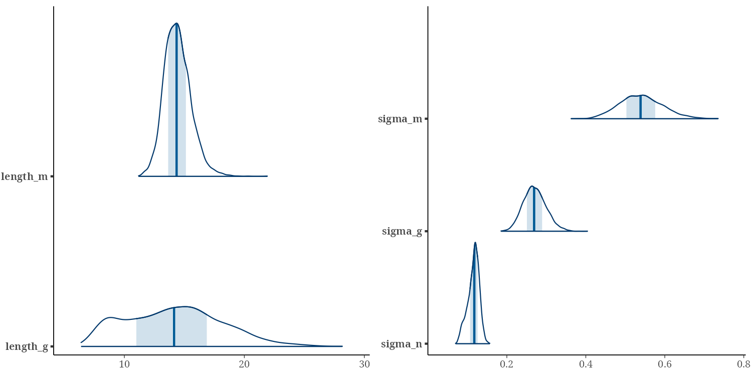
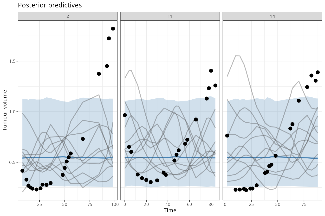
The hierarchical GP with inducing points converged cleanly. R-hat values are close to 1, effective sample sizes are well above 1000, and the chains mix well. Yet the posterior predictive check reveals a poor fit: individual draws are wiggly, while the posterior median is flat. The model is not capturing the strong U-shaped population trend.
Looking at posterior hyperparameters, three things stand out:
The lengthscales are long relative to the trend. With
length_m ≈ 14on a time range of tens of days, the population GP can only produce a few broad bends across the observed range. It cannot produce the sharp downturn and upturn that characterise a U-shape.The population amplitude is small. With
sigma_m ≈ 0.54in standardised log-volume units, the population mean is constrained to vary by only about half a standard deviation. This is not enough to represent a strong U-shape.The patient amplitude is only half the population amplitude. With
sigma_g ≈ 0.27, patient deviations are small. So the model cannot compensate for the weak population trend by letting each patient have their own strong U-shape.
The result is a posterior that spreads its probability mass across many weakly U-shaped or even flat functions. Each draw is wiggly because the GP has enough flexibility to interpolate, but no draw commits to a strong U-shape because the priors and likelihood do not demand it.
The core issue is structural, not computational. A default RBF kernel with weakly informative priors is a general-purpose smoother. It has no built-in preference for a strong global trend. When the data are sparse and noisy, the posterior defaults to a broad distribution over smooth functions rather than concentrating on the trend you expect.
There are principled ways to fix this. The key is to encode the U-shape assumption either through a custom kernel built from exponential basis functions or through a parametric population mean with GP residuals for patient deviations. Both approaches preserve the Bayesian hierarchical framework. The choice depends on whether you prefer flexibility (kernel) or interpretability and stability (parametric mean). We will explain these solutions in future posts.