From Equations to Trajectories: Deterministic Simulation and Stochastic Processes in the Two-Compartment Tumor Model
Systems biology builds mechanistic models in Odinary Differential Equations (ODEs) or Partial Differential Equations (PDEs) from known biology. It derives mathematical equations from chemical reactions, with kinetic parameters describing the rates of these processes.
These ODE models can be simulated deterministically (same initial conditions → same trajectory) or stochastically (adding random fluctuations at each step). The model parameters are often tuned manually without considering identifiability — can we actually estimate them from data? Parameter estimation is largely missing because these models are forward‑facing — they tell you what should happen, not what did happen given messy real‑world measurements.
Statistics, on the other hand, looks backwards. It builds inferential engines from noisy, incomplete observations. Statistics helps us estimate parameters and quantify uncertainty from partially observed data.
In this post, I’ll use a well‑known two‑compartment tumor model to walk from forward deterministic simulation to forward stochastic simulation with different ways of incorporating randomness. And in a follow up post, I will demonstrate how to use state-space models to make the backward inference as well as forward simulation.
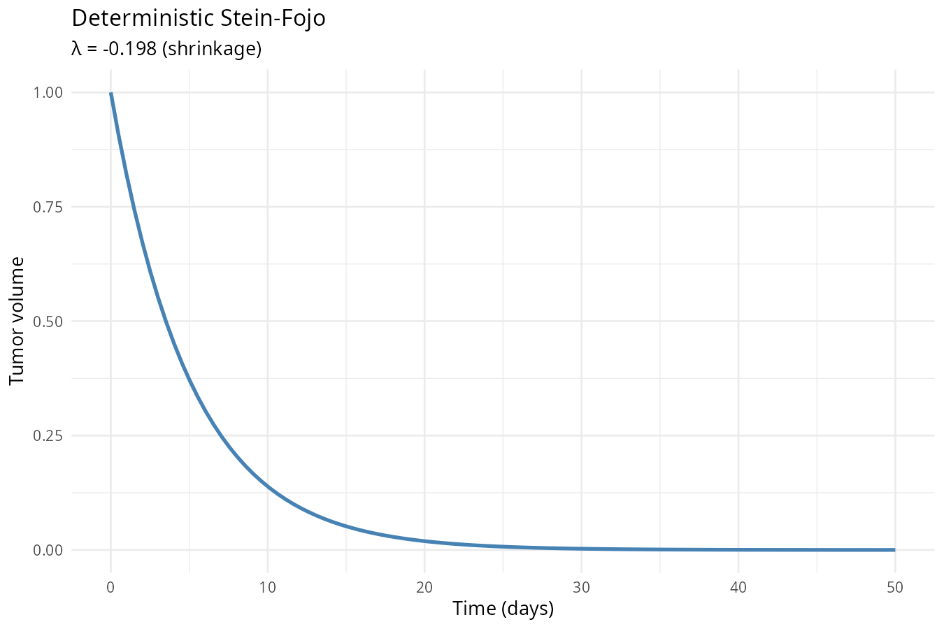
The Stein-Fojo Tumor Model
A tumor is often composed of sensitive (dying under treatment) and resistant (growing despite treatment) cells. The classic Stein‑Fojo model treats the tumor as a single mixed population with fixed sensitive fraction \(f\). This gives monotonic growth or decay depending on the balance of growth and death rates:
\[ \frac{dT}{dt} = f \cdot T \cdot \big(- k_s\big) + (1-f) \cdot T \cdot k_g \]
Where:
- \(T\) = total tumor volume
- \(f\) = fraction of cells that are sensitive to treatment
- \(k_s\) = death rate of sensitive cells
- \(k_g\) = growth rate of resistant cells
The Two-Compartment Tumor Model
However real tumors often show a U‑shaped response (shrink then regrow) because resistance emerges. To capture this, we explicitly model two compartments:
- Sensitive cells \(S\): die under treatment. This is a first-order decay reaction: \[S \xrightarrow{k_s} \emptyset\]
- Resistant cells \(R\): grow (divide) despite treatment. This is a first-order autocatalytic reaction: \[R \xrightarrow{k_g} 2R\]
Applying the law of mass action to these elementary reactions: \[ \begin{aligned} \frac{dS}{dt} &= -k_s S \\ \frac{dR}{dt} &= k_g R \end{aligned} \]
Deterministic Simulation (Forward Propagation)
We treat parameters \((S_0, R_0, k_s, k_g)\) as known. But instead of solving numerically with Euler or Runge‑Kutta (RK4) , we can find analytical solutions because these ODEs are linear:
Initial conditions: \(S(0) = S_0\), \(R(0) = R_0\).
The total volume: \[T(t) = S(t) + R(t) = S_0 e^{-k_s t} + R_0 e^{k_g t}\]
Show R code
# Parameters
S0 <- 0.99
R0 <- 0.01
ks <- 0.2
kg <- 0.05
time <- seq(0, 100, length.out = 200)

S <- S0 * exp(-ks * time)
R <- R0 * exp(kg * time)
T_total <- S + R

df <- data.frame(time = time, Sensitive = S, Resistant = R, Total = T_total) %>%
  tidyr::pivot_longer(-time, names_to = "Compartment", values_to = "Volume")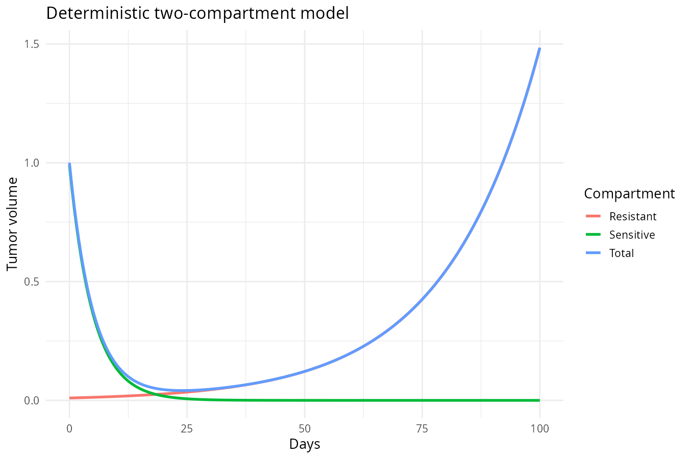
Key insight: This is a forward propagation — given initial states and parameters, you get one answer and no uncertainty.
Solving \(\frac{dS}{dt} = -k_s S\): This is a first‑order linear ODE. By separating variables and integrating \(\int \frac{1}{S} \, dS = \int -k_s \, dt\), we get \(\ln(S) = -k_s t + C\), then \(S = e^{-k_s t + C} = e^C \cdot e^{-k_s t}\). Let \(S_0 = e^C\) (this is the value of \(S\) when \(t=0\)), we obtain \(S(t) = S_0 e^{-k_s t}\). This exponential decay means that each sensitive cell has a constant probability of dying per unit time, independent of the population size. The half‑life \(t_{1/2} = \ln(2)/k_s\) is the time it takes for half the sensitive cells to die.
What are Euler and RK4?
- Euler: The simplest numerical method — step forward using the slope at the beginning of the interval. Fast but can be inaccurate for stiff equations.
- RK4 (4th‑order Runge‑Kutta) : A more accurate method that averages slopes at the beginning, middle, and end of each step. It’s the workhorse of ODE simulation.
Stochastic Simulation (Adding Process Noise)
Multiplicative Noise on the Populations
Reality is messy. Cell can grow and die as random processes. Besides, drug efficacy can vary. We can upgrade our ODE to an SDE (Stochastic Differential Equation). The most common way to write the two‑compartment model as SDEs is to add multiplicative noise directly to each population. This models random fluctuations in cell division and death:
\[ \begin{aligned} dS &= -k_s S \, dt + \sigma_S S \, dW_S \\ dR &= k_g R \, dt + \sigma_R R \, dW_R \end{aligned} \]
Here \(\sigma [ S,D ] \, dW\) is stochastic diffusion — random noise scaled by tumor size. \(\sigma\) represents volatility or relative noise intensity. It measures how much random fluctuation exists relative to the current tumor size. The noise is multiplicative (proportional to \(S\) and \(R\)) because larger tumors have more cells and thus more absolute random variation and this also keeps the populations positive. And \(dW\) is a Wiener process increment (continuous‑time white noise, also called Brownian motion). We can think of \(dW\) as the limit of a random walk where you take infinitesimally small steps at infinitesimally high frequency.
In practice, we can’t work directly with infinitesimals. We approximate the SDE over small discrete time steps \(\Delta t\) and use Euler‑Maruyama approximation (\(\Delta W_t\)) to simulate SDE:
\[ \begin{aligned} S_{t+1} &= S_t - k_s S_t \Delta t + \sigma_S S_t \, \Delta W_{S,t} \\ R_{t+1} &= R_t + k_g R_t \Delta t + \sigma_R R_t \, \Delta W_{R,t} \end{aligned} \]
Where \(\Delta W_t = \epsilon_t \sqrt{\Delta t}\) with \(\epsilon_t \sim \mathcal{N}(0,1)\). So:
\[ \begin{aligned} S_{t+1} &= S_t \left(1 - k_s \Delta t + \sigma_S \epsilon_{S,t} \sqrt{\Delta t}\right) \\ R_{t+1} &= R_t \left(1 + k_g \Delta t + \sigma_R \epsilon_{R,t} \sqrt{\Delta t}\right) \end{aligned} \]
Note: Sampling \(\Delta W_t = \epsilon_t \sqrt{\Delta t}\) with \(\epsilon_t \sim \mathcal{N}(0,1)\) is mathematically equivalent to directly drawing \(\Delta W_t \sim \mathcal{N}(0, \Delta t)\). The former is often used in code because most random number generators provide standard normals (\(\mathcal{N}(0,1)\)) as primitives.
To keep population non‑negative, we can either use a smaller \(\Delta t\) or set a lower bound (e.g., max(..., 0)) after each step. A more elegant solution is to work on the log scale, where the SDE becomes additive and exponentiation guarantees positivity.
Let \(s_t = \log S_t\), \(r_t = \log R_t\). Applying Itô’s lemma:
\[ \begin{aligned} ds_t &= \left(-k_s - \frac{\sigma_S^2}{2}\right) dt + \sigma_S dW_S \\ dr_t &= \left(k_g - \frac{\sigma_R^2}{2}\right) dt + \sigma_R dW_R \end{aligned} \]
Euler-Maruyama on log scale:
\[ \begin{aligned} s_{t+1} &= s_t + \left(-k_s - \frac{\sigma_S^2}{2}\right) \Delta t + \sigma_S \epsilon_{S,t} \, \sqrt{\Delta t} \\ r_{t+1} &= r_t + \left(k_g - \frac{\sigma_R^2}{2}\right) \Delta t + \sigma_R \epsilon_{R,t} \, \sqrt{\Delta t} \end{aligned} \]
Then exponentiate to get \(S\) and \(R\), to ensure positivity:
\[ S_{t+1} = \exp(s_{t+1}), \quad R_{t+1} = \exp(r_{t+1}) \]
Why arithmetic scale can fail: The Euler-Maruyama approximation on the original scale updates \(S\) as \(S_{t+1} = S_t(1 - k_s\Delta t + \sigma_s\epsilon_t\sqrt{\Delta t})\). If the random term \(\sigma_s\epsilon_t\sqrt{\Delta t}\) is sufficiently negative, the factor in parentheses can become negative, driving the population below zero. This is more likely when the time step \(\Delta t\) is large (roughly \(\Delta t > 1/k_s\)). To avoid this, we simulate on the log scale, where the update is additive and exponentiation guarantees positivity.
Show R code
S0 <- 0.99
R0 <- 0.01
ks <- 0.2
kg <- 0.05
sigma_s <- 0.15
sigma_r <- 0.10
dt <- 0.01
n_steps <- 10000
n_sim <- 50

set.seed(42)
S_log <- matrix(NA, nrow = n_steps, ncol = n_sim)
R_log <- matrix(NA, nrow = n_steps, ncol = n_sim)
S_log[1, ] <- log(S0)
R_log[1, ] <- log(R0) # initialise each simulation with the same initial tumour volume

for (i in 2:n_steps) {
  eps_s <- rnorm(n_sim)
  eps_r <- rnorm(n_sim)
  S_log[i, ] <- S_log[i-1, ] + (-ks - sigma_s^2/2) * dt + sigma_s * sqrt(dt) * eps_s
  R_log[i, ] <- R_log[i-1, ] + (kg - sigma_r^2/2) * dt + sigma_r * sqrt(dt) * eps_r
}

S_log<- exp(S_log)
R_log<- exp(R_log)
T_log<-S_log+R_log

df_log <- data.frame(
  time = rep(seq(0, (n_steps-1)*dt, length.out = n_steps), times = n_sim), #repeat whole sequence n_steps times
  sim = rep(1:n_sim, each = n_steps), #repeat each simulation index n_steps times
  volume = as.vector(T_log)
)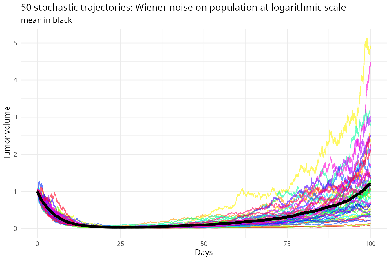
Output: An ensemble of trajectories (Monte Carlo runs).
Insight: This captures intrinsic randomness (process noise) — but still forward only. We haven’t learned anything from data yet.
Multiplicative Noise on the Rates
Biological rates fluctuate due to microenvironment, immune response, and drug efficacy. Instead of adding noise directly to \(S\) and \(R\), we add Wiener noise to the rates. As shown in the following equations, rates are stochastic and noise magnitude is proportional to the current rate. Populations, \(S\) and \(R\) evolve deterministically given the noisy rates (deterministic conditional on rates):
\[ \begin{aligned} dk_s &= \sigma_s k_s \, dW_s \\ dk_g &= \sigma_g k_g \, dW_g \\ dS &= -k_s S \, dt \\ dR &= k_g R \, dt \end{aligned} \]
Based on the Euler‑Maruyama approximation, the rates evolve as:
\[ \begin{aligned} k_{s,t+1} &= k_{s,t} + \sigma_s k_{s,t} \Delta W_{s,t} \\ &= k_{s,t} \left(1 + \sigma_s \epsilon_{s,t} \sqrt{\Delta t}\right) \\ k_{g,t+1} &= k_{g,t} + \sigma_g k_{g,t} \Delta W_{g,t} \\ &= k_{g,t} \left(1 + \sigma_g \epsilon_{g,t} \sqrt{\Delta t}\right) \end{aligned} \]
Where \(\Delta W_t = \epsilon_t \sqrt{\Delta t}\), \(\epsilon_t \sim \mathcal{N}(0,1)\). As in the section above, this can also produce negative rates if \(\epsilon\) is sufficiently negative and \(\Delta t\) is large.
To guarantee positivity of rates, simulate on log scale.
Let \(u_t = \log k_{s,t}\), \(v_t = \log k_{g,t}\). Applying Itô’s lemma to \(du_t\) and \(dv_t\) will introduce a constant drift correction term of \(-\sigma^2/2\) and additive noise:
\[ \begin{aligned} du_t &= -\frac{\sigma_s^2}{2} dt + \sigma_s dW_s \\ dv_t &= -\frac{\sigma_g^2}{2} dt + \sigma_g dW_g \end{aligned} \]
Then, with Euler-Maruyama on log scale of rates and transforming back to the original scale (exponentiating will guarantee positivity), with populations evolving deterministically given the rates at the beginning of the interval:
\[ \begin{aligned} \log k_{s,t+1} &= \log k_{s,t} - \frac{\sigma_s^2}{2} \Delta t + \sigma_s \sqrt{\Delta t} \, \epsilon_{s,t} \\ \log k_{g,t+1} &= \log k_{g,t} - \frac{\sigma_g^2}{2} \Delta t + \sigma_g \sqrt{\Delta t} \, \epsilon_{g,t} \end{aligned} \]
\[ \begin{aligned} k_s &= \exp(\log k_s) \\ k_g &= \exp(\log k_g) \\ S_{t+1} &= S_t - k_{s,t} S_t \Delta t \\ R_{t+1} &= R_t + k_{g,t} R_t \Delta t \end{aligned} \]
Show R code
# Parameters
S0 <- 0.99
R0 <- 0.01
ks0 <- 0.2   # initial sensitive death rate
kg0 <- 0.05  # initial resistant growth rate
sigma_s <- 0.03   # noise on ks
sigma_g <- 0.02  # noise on kg
dt <- 0.01       # time step (days)
n_steps <- 10000   # number of steps
n_sim <- 50      # number of simulations

# Log-scale simulation (rates stay positive)
set.seed(42)

# Initialize
ks <- matrix(NA, nrow = n_steps, ncol = n_sim)
kg <- matrix(NA, nrow = n_steps, ncol = n_sim)
S <- matrix(NA, nrow = n_steps, ncol = n_sim)
R <- matrix(NA, nrow = n_steps, ncol = n_sim)

ks[1, ] <- ks0
kg[1, ] <- kg0
S[1, ] <- S0
R[1, ] <- R0

for (i in 2:n_steps) {
  # Draw noise for each simulation
  eps_s <- rnorm(n_sim)
  eps_g <- rnorm(n_sim)

  # Update logs (additive noise with Itô correction)
  ks[i,] <- log(ks[i-1, ]) - (sigma_s^2 / 2) * dt + sigma_s * sqrt(dt) * eps_s
  kg[i,] <- log(kg[i-1, ]) - (sigma_g^2 / 2) * dt + sigma_g * sqrt(dt) * eps_g

  # Exponentiate to get rates (always positive)
  ks[i,] <- exp(ks[i,])
  kg[i,] <- exp(kg[i,])

  # Update populations (deterministic given rates at start of interval)
  S[i,] <- S[i-1,] - ks[i-1,] * S[i-1,] * dt
  R[i,] <- R[i-1,] + kg[i-1,] * R[i-1,] * dt
}

# Total volume
T_total <- S + R

df_T <- data.frame(
  time = rep(seq(0, (n_steps-1)*dt, length.out = n_steps), times = n_sim), #repeat whole sequence n_steps times
  sim = rep(1:n_sim, each = n_steps), #repeat each simulation index n_steps times
  volume = as.vector(T_total),
  ks = as.vector(ks),
  kg = as.vector(kg)
)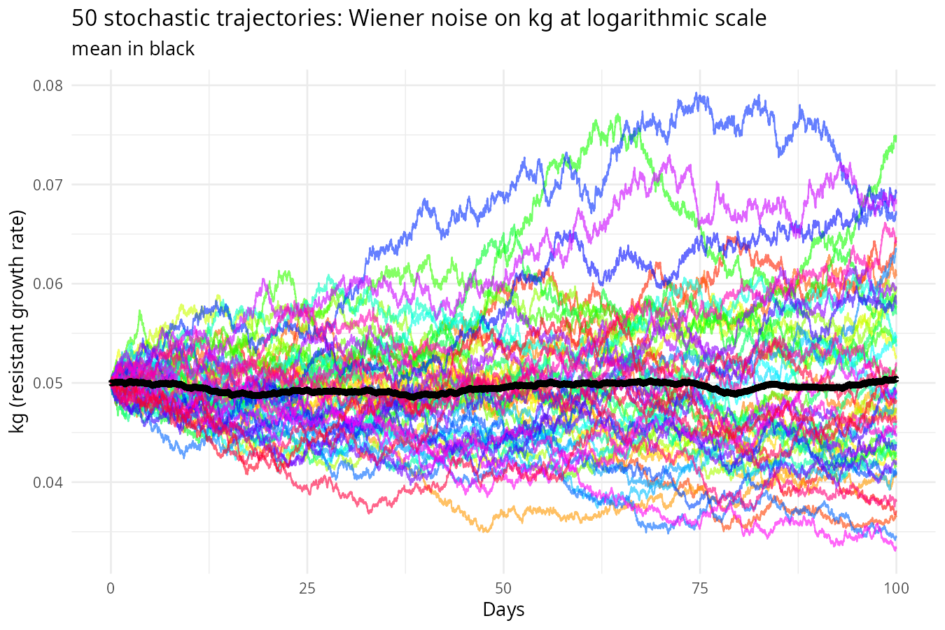
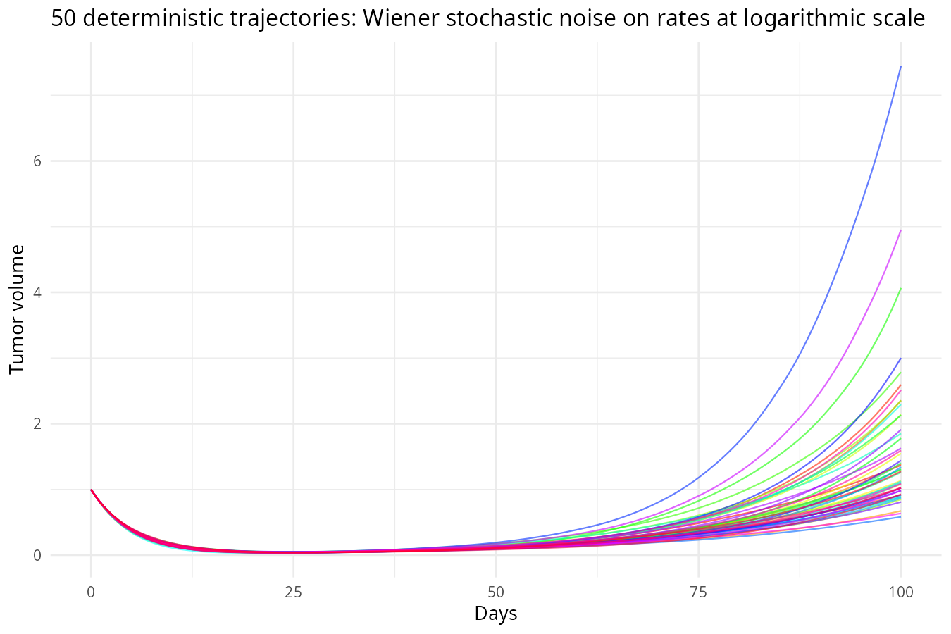
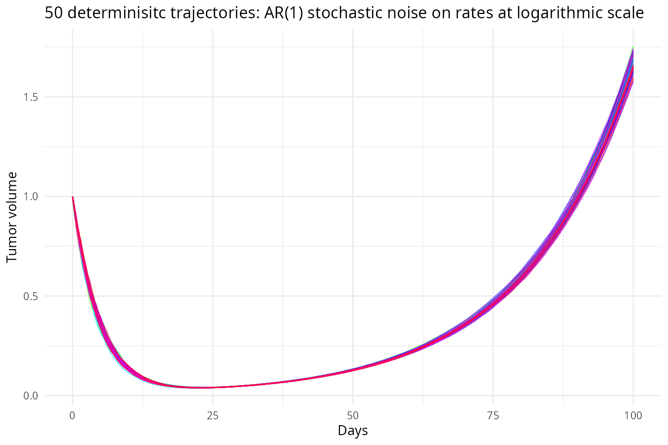
Why noise on rates can bring extreme volatility, but population curve remains smooth: From \(\frac{dS}{dt} = -k_s(t) S\), separation of variables gives \(S(t) = S_0 \exp\left(-\int_0^t k_s(u) du\right)\). Thus \(S\) is an exponential of the integral of the rate. Any random fluctuation in \(k_s\) is integrated and then exponentiated. The fluctuations can indirectly feedback to further changes through current rates (as this is multiplicative noise on rates), leading to large, persistent effects. Therefore,noise on rates accumulates over time, creating large uncertainty in future population sizes and far more volatile population dynamics than noise added directly to the populations.
However, because populations are integrals of the rates, the resulting trajectories are smooth – the integration acts like a low‑pass filter, smoothing out high‑frequency bumps. In contrast, noise added directly to populations makes the curves appear jagged, but the long‑term uncertainty is smaller because the noise does not compound.
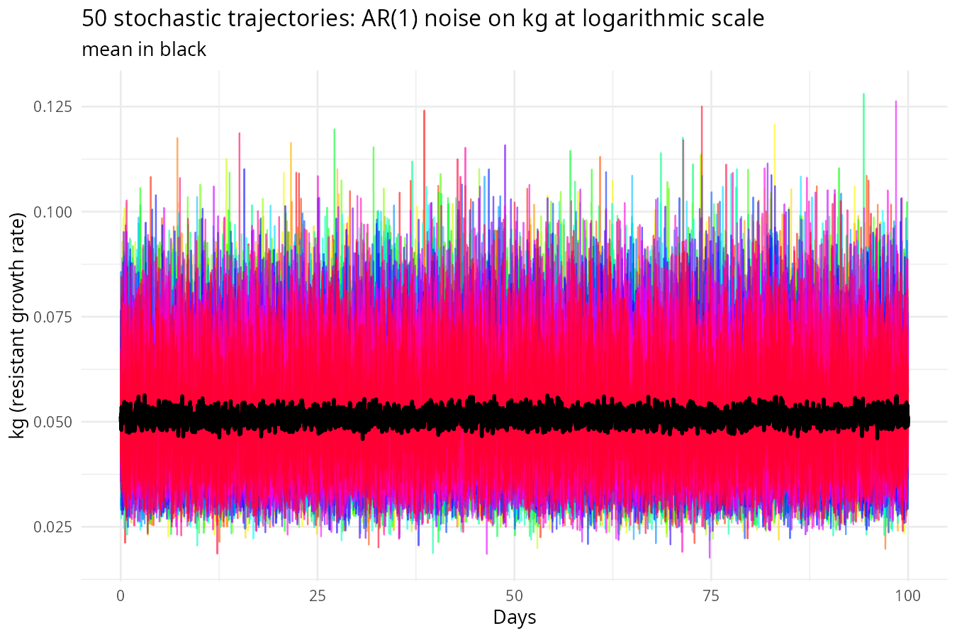
Adding AR(1) Noise on Rates
So far we used Wiener (white) noise on rates: \(dk = \sigma k dW\). This produces rates that are continuous‑time random walks (geometric Brownian motion). The increments are independent, and the rate can drift arbitrarily far.
AR(1) noise (autoregressive of order 1) introduces mean reversion and temporal correlation. This is often more realistic for biological rates:
- Rates (e.g., drug metabolism, immune activity) fluctuate around a baseline.
- They don’t drift to infinity or zero; they revert to a mean.
- Shocks decay exponentially over time.
For rates like \(k_s\) and \(k_g\), AR(1) ensures they stay in a plausible range without external constraints.
The simplest AR(1) on the original scale:
\[ k_t = \mu + \phi (k_{t-1} - \mu) + \epsilon_t, \quad \epsilon_t \sim \mathcal{N}(0, \sigma_w^2) \]
where \(\phi\) models persistence (0 < \(\phi\) < 1 for mean reversion) and \(\mu\) is the long‑term mean. However, this can produce negative rates if \(\epsilon_t\) is large and negative. To ensure positivity, we model on the log scale:
Log‑Scale AR(1) for Rates
Let \(u_t = \log k_t\). Assume an AR(1) process on \(u_t\), so we directly define the AR(1) on the log rate, and no Itô correction is needed because this is a discrete‑time model:
\[ u_t = \mu_u + \phi (u_{t-1} - \mu_u) + \eta_t, \quad \eta_t \sim \mathcal{N}(0, \sigma_u^2) \]
Then \(k_t = \exp(u_t)\) is always positive.
Full two‑compartment model with AR(1) on log rates:
Let \(u_t = \log k_{s,t}\), \(v_t = \log k_{g,t}\), and populations \(S_t\), \(R_t\) will inheritate log-normal noise from the AR(1) processes.
\[ \begin{aligned} u_t &= \mu_u + \phi_u (u_{t-1} - \mu_u) + \eta_{u,t}, \quad \eta_{u,t} \sim \mathcal{N}(0, \sigma_u^2) \\ v_t &= \mu_v + \phi_v (v_{t-1} - \mu_v) + \eta_{v,t}, \quad \eta_{v,t} \sim \mathcal{N}(0, \sigma_v^2) \\ S_t &= S_{t-1} - \exp(u_{t-1}) \, S_{t-1} \Delta t \\ R_t &= R_{t-1} + \exp(v_{t-1}) \, R_{t-1} \Delta t \end{aligned} \]
Show R code
S0 <- 0.99
R0 <- 0.01
ks0 <- 0.2   # initial sensitive death rate
kg0 <- 0.05  # initial resistant growth rate
mu_u <- log(ks0)   # mean log ks
mu_v <- log(kg0)  # mean log kg
phi_u <- 0.8
phi_v <- 0.7
sigma_u <- 0.2
sigma_v <- 0.15

dt <- 0.01
n_steps <- 10000
n_sim <- 50      # number of simulations

set.seed(42)

# Initialize
ks <- matrix(NA, nrow = n_steps, ncol = n_sim)
kg <- matrix(NA, nrow = n_steps, ncol = n_sim)
u <- matrix(NA, nrow = n_steps, ncol = n_sim)
v <- matrix(NA, nrow = n_steps, ncol = n_sim)
S <- matrix(NA, nrow = n_steps, ncol = n_sim)
R <- matrix(NA, nrow = n_steps, ncol = n_sim)

ks[1, ] <- ks0
kg[1, ] <- kg0
u[1, ] <- mu_u
v[1, ] <- mu_v
S[1, ] <- S0
R[1, ] <- R0

for (t in 2:n_steps) {
  u[t,] <- mu_u + phi_u * (u[t-1,] - mu_u) + sigma_u * rnorm(n_sim)
  v[t,] <- mu_v + phi_v * (v[t-1,] - mu_v) + sigma_v * rnorm(n_sim)
  ks[t,] <- exp(u[t,])
  kg[t,] <- exp(v[t,])
  S[t,] <- S[t-1,] - ks[t-1,] * S[t-1,] * dt
  R[t,] <- R[t-1,] + kg[t-1,] * R[t-1,] * dt
}

T_total<- S + R

df_T <- data.frame(
  time = rep(seq(0, (n_steps-1)*dt, length.out = n_steps), times = n_sim), #repeat whole sequence n_steps times
  sim = rep(1:n_sim, each = n_steps), #repeat each simulation index n_steps times
  volume = as.vector(T_total),
  ks = as.vector(ks),
  kg = as.vector(kg)
)