From Trajectories to Beliefs: State-Space model and Statistical Inference of the Two-Compartment Tumor Model

systems biology

Stochastic Differential Equations

SDE

AR(1)

statistics

inference

state-space model

bayesian statistics

hierarchical bayesian model

stan

advanced

Published

July 5, 2026

In a previous post, we explored the two-compartment tumour growth model, simulating it both deterministically and stochastically. This model captures the dynamics of sensitive and resistant tumor cell populations under treatment, with parameters controlling growth rates and drug sensitivity. However, that was a forward simulation — we started with known parameters and generated trajectories.

Sensitive cells \(S\): die under treatment. This is a first-order decay reaction: \[S \xrightarrow{k_s} \emptyset\]
Resistant cells \(R\): grow (divide) despite treatment. This is a first-order autocatalytic reaction: \[R \xrightarrow{k_g} 2R\]

In this post, we flip the direction: from forward simulation to backward inference. We’ll consider a continuous‑state, discrete‑time state‑space model. The true tumor state (sensitive and resistant populations) can be any positive real numbers, but we only observe total volume at discrete clinical visits. The evolution between visits follows the two‑compartment dynamics with AR(1) noise on the log rates.

For purists: The true biological process is continuous‑time, but discrete‑time models are standard in statistical inference because data arrives at discrete times. If you need arbitrary measurement times, look into continuous‑discrete Kalman filtering.

A state-space model describes a system that evolves over time using two equations: a state equation for the hidden (unobserved) dynamics, and an observation equation for the noisy measurements we actually see. The term “space” comes from mathematics and control theory: the state of a system — the minimal set of variables needed to fully describe it at any moment — lives in an abstract space called the state space. This space contains all possible values the state can take. For a tumor, the state might be \((\log S, \log R)\), which lives in a two‑dimensional real space \(\mathbb{R}^2\). Even though we can’t see this “space” directly, the model allows the state to move through it over time, guided by the state equation. So “space” doesn’t refer to physical space, but to the mathematical space of all possible configurations of the system.

State Equation with AR(1) Process Noise on Log Rates

The two‑compartment model has two latent rates: \(k_s\) (sensitive death rate) and \(k_g\) (resistant growth rate). We add process noise to these rates, not directly to the populations. This is more biologically plausible: rates fluctuate due to changing microenvironment, immune activity, or drug penetration.

To keep rates positive and allow temporal correlation, we model the log rates as AR(1) processes:

Let \(u_t = \log k_{s,t}\) and \(v_t = \log k_{g,t}\).

\[ \begin{aligned} u_t &= \mu_u + \phi_u (u_{t-1} - \mu_u) + \eta_{u,t}, \quad \eta_{u,t} \sim \mathcal{N}(0, \sigma_u^2) \\ v_t &= \mu_v + \phi_v (v_{t-1} - \mu_v) + \eta_{v,t}, \quad \eta_{v,t} \sim \mathcal{N}(0, \sigma_v^2) \end{aligned} \]

Where:
- \(\mu_u\), \(\mu_v\) are the long‑term means of the log rates
- \(\phi_u\), \(\phi_v\) control persistence (close to 1 = slow mean reversion)
- \(\sigma_u^2\), \(\sigma_v^2\) are the innovation variances

Why AR(1) on log rates? This guarantees \(k_s, k_g > 0\), introduces temporal correlation, and keeps the rates mean‑reverting (they don’t drift to infinity or zero).

The populations then evolve deterministically given these rates:

\[ \begin{aligned} S_t &= S_{t-1} - \exp(u_{t-1}) \, S_{t-1} \Delta t \\ R_t &= R_{t-1} + \exp(v_{t-1}) \, R_{t-1} \Delta t \end{aligned} \]

Note on timing: We use the rate from the beginning of the interval (\(u_{t-1}\), \(v_{t-1}\)) to update populations. This is the standard explicit Euler scheme and is causal (no future information needed).

No Itô correction needed here. Unlike the single‑population Stein‑Fojo where we transformed the SDE for \(T\), here we directly model the log rates as discrete‑time AR(1) processes. This is a statistical model choice, not a discretization of a continuous‑time SDE for the rates.

Observation Equation

We don’t see \(S_t\) and \(R_t\) separately — only the total tumour volume \(T_t = S_t + R_t\) from CT scans, with measurement error. Therefore, the noise is added to total tumour because we can only meausre total tumour.

On the log scale, a common and convenient assumption is that measurement errors are additive and Gaussian:

\[ y_t = \log(S_t + R_t) + \nu_t, \quad \nu_t \sim \mathcal{N}(0, R_{\text{obs}}) \]

where \(y_t\) is the observed log‑total‑volume and \(R_{\text{obs}}\) is the measurement error variance.

Why additive noise on the log scale or multiplicative noise on the original scale? On the log scale, it’s natural to assume additive Gaussian measurement error. Transforming back to the original scale gives \(Y_t = T_t \times e^{\nu_t}\), which is multiplicative log-normal noise. This matches clinical reality: measurement error scales with tumor size (e.g., ±5% of volume). Additive noise on the original scale would allow negative volumes and wouldn’t reflect the proportional nature of CT measurement error.

Model Hierarchy and Simplifications

In order to borrow strength across patients, improving estimations of parameters, we built a hierarchical bayesian model with simplifications for parameters. Our model is hierarchical, meaning we estimate parameters at two levels:

Population level: Shared across all patients (e.g., mu_phi, sigma_phi).
Patient level: Allowed to vary per patient (e.g., phi[i], sigma[i], mu_u[i]).

This structure allows the model to learn from all patients while still capturing individual differences.

Same \(\phi\) for \(u\) and \(v\) (Persistence)

The persistence parameter \(\phi_i\) controls how quickly fluctuations in the log-rates decay. We assume that for a given patient, the speed of mean reversion is the same for the sensitive death rate (\(u\)) and the resistant growth rate (\(v\)). This is a simplification, but it is biologically reasonable if both rates are influenced by the same underlying factors (e.g., the tumor microenvironment or drug penetration).

Same \(\sigma\) for \(u\) and \(v\) (Innovation Standard Deviation)

Similarly, the innovation standard deviation \(\sigma_i\) controls the magnitude of random fluctuations. We assume that the typical size of a random shock is the same for both rates within a patient. This reduces the number of parameters and improves identifiability, while still allowing each patient to have their own level of volatility.

What Varies: The Actual Noise (\(\epsilon\))

Although \(\phi_i\) and \(\sigma_i\) are shared, the actual random shocks applied to \(u\) and \(v\) are independent. At each time point \(t\):

For \(u\): u[i, t] = mu_u[i] + phi[i] * (u[i, t-1] - mu_u[i]) + sigma[i] * epsilon_u[i, t]
For \(v\): v[i, t] = mu_v[i] + phi[i] * (v[i, t-1] - mu_v[i]) + sigma[i] * epsilon_v[i, t]

Here, epsilon_u[i, t] and epsilon_v[i, t] are independent standard normal draws. This means that even though the scale of the noise (\(\sigma_i\)) is the same, the direction and timing of fluctuations are different for the two rates. This allows the model to capture independent biological events (e.g., a sudden drop in sensitive cells due to a drug pulse, while resistant cells continue growing steadily).

Where Does `R_obs` Fit?

R_obs is the observation noise variance — it accounts for measurement error in the observed log-total-volume. It is shared across all patients and all time points, meaning we assume the CT scan measurement error has the same magnitude for every patient at every visit.

This is a simplifying assumption. In practice, you could allow R_obs to vary by patient or by time, but that would add complexity and reduce identifiability.

Complete Parameter Hierarchy

Show Population level (hyperparameters) table

Parameter	Description	Stan declaration
`mu_mu_u`	Population mean of patient-level mean sensitive death rate	`real mu_mu_u`
`mu_mu_v`	Population mean of patient-level mean resistant growth rate	`real mu_mu_v`
`sigma_mu_u`	Between-patient SD for mean sensitive death rates	`real<lower=0> sigma_mu_u`
`sigma_mu_v`	Between-patient SD for mean resistant growth rates	`real<lower=0> sigma_mu_v`
`mu_phi`	Population mean of patient-level persistence (on logit scale)	`real mu_phi`
`sigma_phi`	Between-patient SD for persistence	`real<lower=0> sigma_phi`
`mu_sigma`	Population mean of patient-level innovation SD (on log scale)	`real mu_sigma`
`sigma_sigma`	Between-patient SD for innovation SD	`real<lower=0> sigma_sigma`
`mu_f0`	Population mean of patient-level initial sensitive fraction (on logit scale)	`real mu_f0`
`sigma_f0`	Between-patient SD for initial sensitive fraction	`real<lower=0> sigma_f0`
`R_obs`	Observation noise (shared across all patients and time points)	`real<lower=0> R_obs`

Show Patient level (individual parameters): table

Parameter	Description	Transformed from
`mu_u[i]`	Mean log sensitive death rate for patient `i`	`mu_mu_u + sigma_mu_u * mu_u_raw[i]`
`mu_v[i]`	Mean log resistant growth rate for patient `i`	`mu_mu_v + sigma_mu_v * mu_v_raw[i]`
`phi[i]`	Persistence (shared between \(u\) and \(v\)) for patient `i`	`2inv_logit(mu_phi + sigma_phiphi_raw[i]) - 1`
`sigma[i]`	Innovation SD (shared between \(u\) and \(v\)) for patient `i`	`exp(mu_sigma + sigma_sigma*sigma_raw[i])`
`f0[i]`	Initial sensitive fraction for patient `i`	`inv_logit(mu_f0 + sigma_f0*f0_raw[i])`

Show Latent states (time-varying, patient-specific): table

Parameter	Description	Stan type
`u[i, t]`	Log sensitive death rate at time \(t\) for patient \(i\)	`matrix[N, T] u`
`v[i, t]`	Log resistant growth rate at time \(t\) for patient \(i\)	`matrix[N, T] v`
`ks[i, t]`	Sensitive death rate (original scale)	`matrix[N, T] ks = exp(u)`
`kg[i, t]`	Resistant growth rate (original scale)	`matrix[N, T] kg = exp(v)`
`S[i, t]`	Sensitive population (fraction of total)	`matrix[N, T] S`
`R[i, t]`	Resistant population (fraction of total)	`matrix[N, T] R`
`T_total[i, t]`	Total tumor volume (relative to baseline)	`matrix[N, T] T_total = S + R`
`log_T_total[i, t]`	Log total tumor volume	`matrix[N, T] log_T_total = log(T_total)`
`y_pred[i, t]`	Posterior predictive draw (log scale, with noise)	`normal_rng(log_T_total, sqrt(R_obs))`
`y_pred_orig[i, t]`	Posterior predictive draw (original scale, with noise)	`exp(y_pred)`

Model and Inference

Stan Model

Show Stan code

data {
  int<lower=1> N;              // number of patients
  int<lower=1> T;              // number of observations per patient (balanced)
  real y[N, T];                // observed log total volume
  real dt;                     // time step between observations
}
parameters {
  // Population-level hyperparameters for log rates
  real mu_mu_u;                // population mean of mu_u
  real mu_mu_v;                // population mean of mu_v
  real<lower=0> sigma_mu_u;    // between-patient SD for mu_u
  real<lower=0> sigma_mu_v;    // between-patient SD for mu_v

  // Population hyperparameters for phi (persistence)
  real mu_phi;                 // mean of phi (on logit scale for unbounded)
  real<lower=0> sigma_phi;     // SD of phi
  // Note: we use logit transform to keep phi in (-1,1)
  
  // Population hyperparameters for sigma (innovation SD)
  //  sigma is modelled on log scale, log(sigma)~N(). So sigma~lognormal() always positive.
  real mu_sigma;               // mean of sigma (log scale for positivity)
  real<lower=0> sigma_sigma;   // SD of sigma
  
  // Population hyperparameters for f0 (initial sensitive fraction)
  real mu_f0;                  // logit scale
  real<lower=0> sigma_f0;
  
  // Patient-level random effects
  vector[N] mu_u_raw;
  vector[N] mu_v_raw;
  vector[N] phi_raw;           // for logit(phi)
  vector[N] sigma_raw;         // for log(sigma)
  vector[N] f0_raw;
  
  // Observation noise (shared across patients)
  real<lower=0> R_obs;
  
  // Latent states (every time point) per patient (non-centered)
  vector[N * T] u_raw;
  vector[N * T] v_raw;

}
transformed parameters {
  // Patient-level means
  vector[N] mu_u = mu_mu_u + sigma_mu_u * mu_u_raw;
  vector[N] mu_v = mu_mu_v + sigma_mu_v * mu_v_raw;
  
  // phi: transformed from logit scale to (-1, 1)
  vector[N] phi = 2* inv_logit(mu_phi + sigma_phi * phi_raw) - 1;
  
  // sigma: transformed from log scale to positive
  vector[N] sigma = exp(mu_sigma + sigma_sigma * sigma_raw);

  // Patient-level initial sensitive fractions (constrained to [0,1]), inv_logit is logistic function and logit(p)=log(p/1-p)
  vector[N] f0 = inv_logit(mu_f0 + sigma_f0 * f0_raw);
  
  // Initialize matrices for latent states and derived quantities
  matrix[N, T] u;          // log ks per patient and time
  matrix[N, T] v;          // log kg per patient and time
  matrix[N, T] ks;         // sensitive death rate
  matrix[N, T] kg;         // resistant growth rate
  matrix[N, T] S;          // sensitive population
  matrix[N, T] R;          // resistant population
  matrix[N, T] T_total;    // total volume
  matrix[N, T] log_T_total; // log total volume
  
  // Reconstruct AR(1) processes for each patient
  for (i in 1:N) {
    // Starting Indices for each patient for u_raw and v_raw
    int start = (i-1) * T + 1;
    // int end = i * T;
    
    // Extract patient's raw draws. segment extract a subvector length T start from start
    vector[T] u_raw_i = segment(u_raw, start, T);
    vector[T] v_raw_i = segment(v_raw, start, T);
    
    // AR(1) for u (log ks), at first time point, then following time points
    u[i, 1] = mu_u[i] + sigma[i] * u_raw_i[1];
    for (t in 2:T) {
      u[i, t] = mu_u[i] + phi[i] * (u[i, t-1] - mu_u[i]) + sigma[i] * u_raw_i[t];
    }
    
    // AR(1) for v (log kg)
    v[i, 1] = mu_v[i] + sigma[i] * v_raw_i[1];
    for (t in 2:T) {
      v[i, t] = mu_v[i] + phi[i] * (v[i, t-1] - mu_v[i]) + sigma[i] * v_raw_i[t];
    }
    
    // Transform to rates
    ks[i] = exp(u[i]);
    kg[i] = exp(v[i]);
    
    // Population dynamics (deterministic given rates)
    S[i, 1] = f0[i];
    R[i, 1] = 1 - f0[i];
    T_total[i, 1] = S[i, 1] + R[i, 1];
    log_T_total[i, 1] = log(T_total[i, 1]);
    
    for (t in 2:T) {
      // use fmax to make sure S, R never goes below 1e-10  
      S[i, t] = fmax(S[i, t-1] - ks[i, t-1] * S[i, t-1] * dt, 1e-10);
      R[i, t] = fmax(R[i, t-1] + kg[i, t-1] * R[i, t-1] * dt, 1e-10);
      // use fmin to make sure T_total is not infinate
      T_total[i, t] = fmin(S[i, t] + R[i, t],1e10);
      log_T_total[i, t] = log(T_total[i, t]);
    }
  }
}
model {
  // Hyperpriors
  // log rates
  mu_mu_u ~ normal(log(0.3), 0.5);
  mu_mu_v ~ normal(log(0.05), 0.5);
  sigma_mu_u ~ cauchy(0, 0.2);
  sigma_mu_v ~ cauchy(0, 0.1);
  
  // phi: logit scale priors (mu_phi ~ 0.85 on logit = logit(0.7))
  mu_phi ~ normal(0.85, 0.5);    // 95% CI: expit(0.85) ≈ 0.7
  sigma_phi ~ cauchy(0, 0.2);
  
  // sigma: log scale priors (mu_sigma ~ log(0.15) ≈ -1.9)
  mu_sigma ~ normal(-1.9, 0.5);  // log(0.15)
  sigma_sigma ~ cauchy(0, 0.2);

  // f0
  mu_f0 ~ normal(2.2, 0.5);    // logit scale, logit(0.9)=2.2
  sigma_f0 ~ cauchy(0, 0.3);
  
  R_obs ~ cauchy(0, 0.05);
  
  // Patient-level random effects (non-centered, auxiliary parameter)
  mu_u_raw ~ std_normal();
  mu_v_raw ~ std_normal();
  phi_raw ~ std_normal();
  sigma_raw ~ std_normal();
  f0_raw ~ std_normal();
  
  // Latent states (all time points)(non-centered AR(1))
  u_raw ~ std_normal();
  v_raw ~ std_normal();
  
  // Likelihood
  for (i in 1:N) {
    for (t in 1:T) {
      // observation y[i,t] is on log scale with additive noise
      // the latent state at each time points represent the mean with additive noise
      y[i, t] ~ normal(log_T_total[i, t], sqrt(R_obs));
    }
  }
}
generated quantities {
  // Posterior predictive draws (including observation noise)
  matrix[N, T] y_pred;
  matrix[N, T] y_pred_orig;

  for (i in 1:N) {
    for (t in 1:T) {
      // Generate new observations with observation noise
      y_pred[i, t] = normal_rng(log_T_total[i, t], sqrt(R_obs));
      // Transform to original scale (optional)
      y_pred_orig[i, t] = exp(y_pred[i, t]);
    }
  }
}

Measurement replicates: In most clinical settings, there is only one tumor measurement per patient per visit (e.g., a single CT scan). Our model assumes this common case: one noisy observation per time point. If multiple measurements were available (e.g., two radiologists measuring the same scan), we could extend the observation model to estimate measurement error variance, \(R_{\text{obs}}\), directly from the replicates.

Multiple patients: This Stan model above is for multiple patients with hierarchical priors (partial pooling) to share information across patients. With typical trial data (5-20 observations per patient), hierarchical models improve estimation, especially for patients with sparse data.

Priors: We use half-Cauchy priors for standard deviation parameters (constrained to be positive via real<lower=0>). The Cauchy distribution has heavy tails, making it a robust weakly informative choice. For hyper-priors on log-rate means (mu_mu_u, mu_mu_v), normal priors are appropriate — they can be negative because log rates are often less than zero.

Truncated priors in Stan: When we declare real<lower=0> sigma_mu_u; and then assign sigma_mu_u ~ cauchy(0, 0.2);, Stan automatically interprets this as a truncated Cauchy distribution — the prior density is renormalized to integrate to 1 over positive values only. We don’t need to manually adjust for the negative part; Stan handles it internally. This is one of the conveniences of using a probabilistic programming language like Stan.

Inference, Posterior Sampling and Prediction

Show R code

# Simulate longitudinal tuour sizes of N patients 
# ......

# Prepare data for Stan model
stan_data_fit <- list(
  N = N_patients,
  T = T_obs,
  y = y_sim_norm,   # normalized observed log total volume
  dt = dt
)

# Fit inference model
# initial value to make sure no extreme values are explored
init_func <- function() {
  list(
    mu_mu_u = log(0.3),
    mu_mu_v = log(0.05),
    sigma_mu_u = 0.2,
    sigma_mu_v = 0.1,
    mu_phi = 0.85,
    sigma_phi = 0.2,
    mu_sigma = -1.9,
    sigma_sigma = 0.2,
    mu_f0 = 2.2,
    sigma_f0 = 0.3,
    R_obs = 0.05,
    mu_u_raw = rep(0, N_patients),
    mu_v_raw = rep(0, N_patients),
    phi_raw = rep(0, N_patients),
    sigma_raw = rep(0, N_patients),
    f0_raw = rep(0, N_patients),
    u_raw = rep(0, N_patients * T_obs),
    v_raw = rep(0, N_patients * T_obs)
  )
}

fit_inference <- stan(
  file = paste0(current_dir,"/state-space-AR1.stan"),
  data = stan_data_fit,
  init = init_func,
  iter = 2000,
  warmup = 1000,
  chains = 4,
  control = list(adapt_delta = 0.95,
                  max_treedepth = 12)
)

Tuning adapt_delta: Stan’s NUTS sampler adapts its step size to achieve a target acceptance rate set by adapt_delta. The default is 0.8. For complex models like our two‑compartment state‑space model, we often increase adapt_delta to 0.95 to avoid divergent transitions and ensure accurate posterior exploration. This slows down sampling but improves reliability. If you see warnings about divergent transitions, increase adapt_delta gradually (e.g., 0.85, 0.9, 0.95) until they disappear.

Tuning max_treedepth: limits how many steps the sampler can take before stopping and proposing a new state. Increasing it from the default (10) allows the sampler to explore more complex posterior geometries, especially when parameters are strongly correlated. This helps reduce divergences and improves mixing.

Assessed convergence using standard Stan diagnostics:

Diagnostic Threshold

R‑hat < 1.05

Effective sample size (n_eff) > 100 (ideally > 400)

Divergent transitions < 1% of total transitions (total number of post-warmup iterations across all chains combined)

Tree depth < max_treedepth

Diagnostic	Threshold
R‑hat	< 1.05
Effective sample size (n_eff)	> 100 (ideally > 400)
Divergent transitions	< 1% of total transitions (total number of post-warmup iterations across all chains combined)
Tree depth	< max_treedepth

Prior and Posterior distributions of key parameters

Posterior predictive on tumor volume, overlay with simulated patients’ data

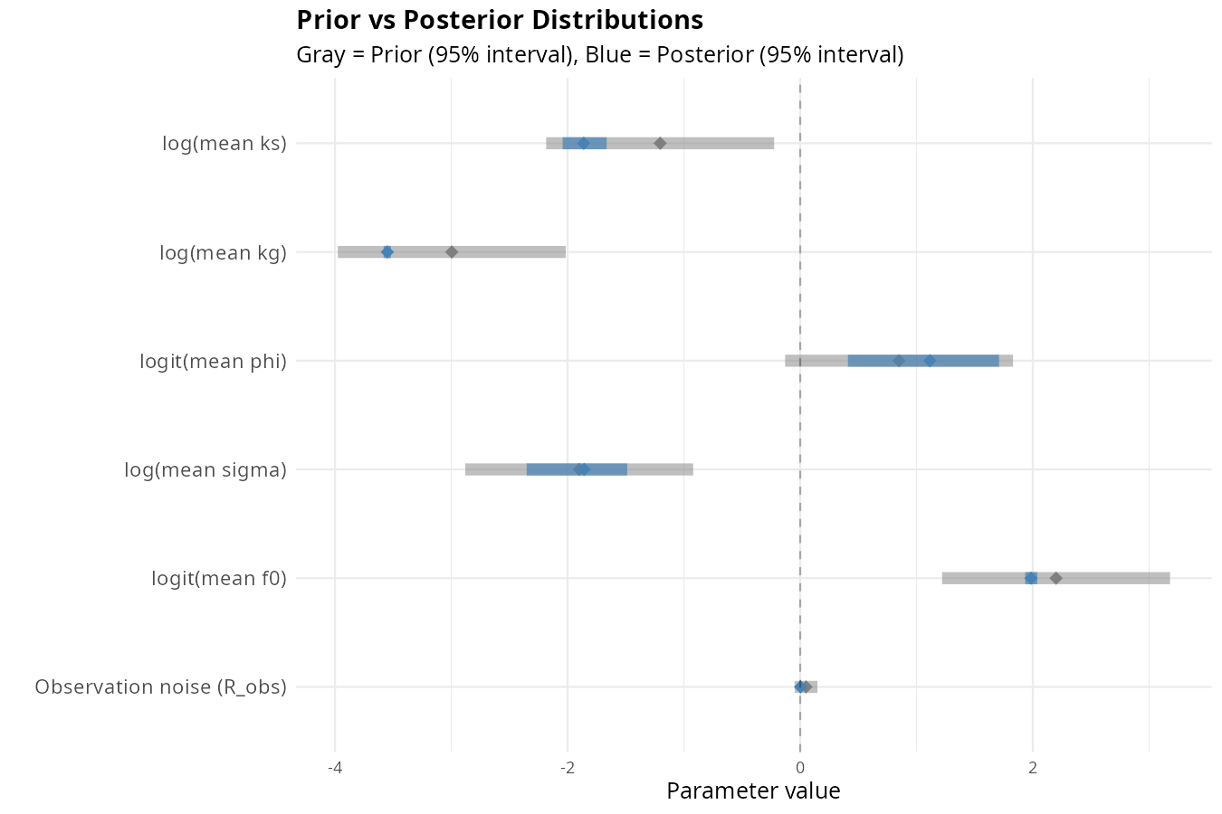
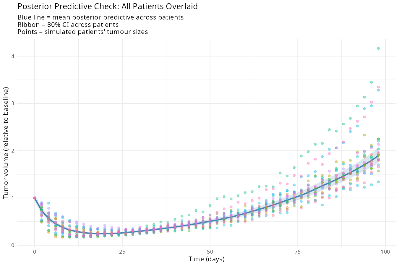
Forward Simulation from the Posterior

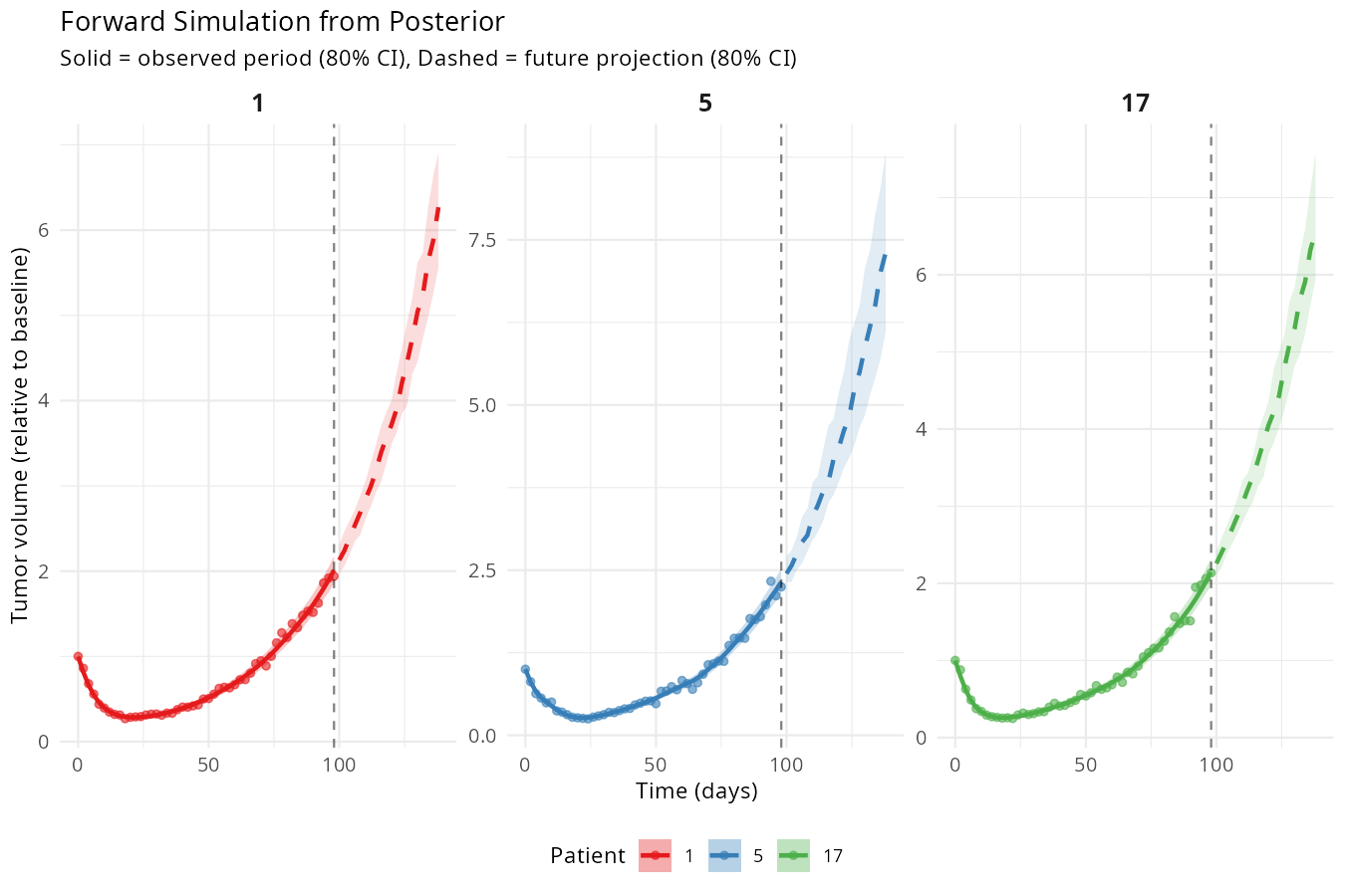
Once we have the posterior, we can simulate forward — not just one trajectory, but a distribution of possible futures for each patient:

Show R code

# load posterior draws
post <- rstan::extract(fit_inference)

# random selection of patients within the total 20 patients
set.seed(42)  # for reproducibility
selected_patients <- sample(1:20, 3)
n_sim_draws <-100
raw_indices <- sample(1:n_draws, n_sim_draws)
T_forward <-20
dt <- 2

# for one patient and one posterior draw, simulate forward in time
simulate_forward <- function(patient_idx, draw_idx, T_forward, dt) {
  # Extract parameters
  mu_u <- post$mu_u[draw_idx, patient_idx]
  mu_v <- post$mu_v[draw_idx, patient_idx]
  phi <- post$phi[draw_idx, patient_idx]
  sigma <- post$sigma[draw_idx, patient_idx]
  R_obs <- post$R_obs[draw_idx]  # Extract observation noise for this draw
  
  # Starting state (last observed latent state)
  u_curr <- post$u[draw_idx, patient_idx, T_obs]
  v_curr <- post$v[draw_idx, patient_idx, T_obs]
  S_curr <- post$S[draw_idx, patient_idx, T_obs]
  R_curr <- post$R[draw_idx, patient_idx, T_obs]
  
  # Initialize vectors for latent and observed volumes
  T_forward_latent <- numeric(T_forward)
  T_forward_observed <- numeric(T_forward)
  
  for (t in 1:T_forward) {
    # 1. Evolve latent state
    u_curr <- mu_u + phi * (u_curr - mu_u) + sigma * rnorm(1)
    v_curr <- mu_v + phi * (v_curr - mu_v) + sigma * rnorm(1)
    
    ks <- exp(u_curr)
    kg <- exp(v_curr)
    
    S_curr <- max(S_curr - ks * S_curr * dt, 1e-10)
    R_curr <- max(R_curr + kg * R_curr * dt, 1e-10)
    
    # 2. Latent (true) total volume
    T_latent <- S_curr + R_curr
    T_forward_latent[t] <- T_latent
    
    # 3. Add observation noise (on log scale) to get predicted observed volume
    log_T_latent <- log(T_latent)
    log_T_observed <- log_T_latent + rnorm(1, 0, sqrt(R_obs))
    T_forward_observed[t] <- exp(log_T_observed)
  }
  
  # Return both latent and observed predictions
  return(list(latent = T_forward_latent, observed = T_forward_observed))
}

# Initialize arrays to store forward simulations
# Dimensions: [n_sim_draws, T_forward, n_selected_patients]
forward_sims <- array(NA, dim = c(n_sim_draws, T_forward, length(selected_patients)))

for (p in 1:length(selected_patients)) {
  patient <- selected_patients[p]
  
  for (i in 1:n_sim_draws) {
    forward_sims[i, , p] <- simulate_forward(patient, draw_indices[i], T_forward, dt)$observed
  }
}

Forward predictions from 100 posterior draws per patient

Limitations and Future Directions

While our two‑compartment state‑space model successfully demonstrates the workflow from mechanistic modeling to statistical inference, several limitations and avenues for improvement deserve mention.

Unrealistic Unlimited Growth: Saturation and Carrying Capacity

A key limitation of our model is the assumption of exponential growth for the resistant compartment:

\[\frac{dR}{dt} = k_g R\]

This allows tumor volume to grow without bound, which is biologically unrealistic. In reality, tumor growth is constrained by nutrient availability, space, and immune response — typically modeled with a carrying capacity:

Approach	Formula	Annotation	Where to add AR(1)	Pros	Cons
1. Decaying \(k_g\)	\(k_g(t) = k_{g,0} \cdot e^{-\gamma t}\)	Growth rate decays exponentially over time; \(\gamma\) = decay rate.	On \(k_{g,0}\) (patient‑level) OR on \(\log k_g(t)\) (time‑varying).	Simple, few parameters, directly extends current model.	No hard upper bound; growth never truly stops.
2. Gompertz	\(\frac{dR}{dt} = k_g \cdot R \cdot \log\left(\frac{K}{R}\right)\)	Growth slows as \(R\) approaches carrying capacity \(K\); \(k_g\) = initial growth rate.	On \(k_g\) (patient‑level or time‑varying) OR on \(K\) (patient‑specific).	Biologically established; enforces a hard upper bound.	Adds parameter \(K\); may be hard to identify with short time series.
3. Emax (Michaelis‑Menten)	\(\frac{dR}{dt} = k_g \cdot R \cdot \frac{1}{1 + (R/K)^\gamma}\)	Growth modulated by saturating function; \(K\) = half‑saturation size, \(\gamma\) = steepness.	On \(k_g\) (over time) OR on \(K\) or \(\gamma\) (patient‑specific).	Flexible; can approximate Gompertz or logistic shapes.	More parameters; requires strong priors to avoid overfitting.

Identifiability: \(k_s\) and \(k_g\) Trade‑off

A persistent challenge in our model is the identifiability of \(k_s\) and \(k_g\) from total volume alone. Many combinations of \((k_s, k_g)\) can produce similar total volume trajectories, especially when both rates fluctuate. A better parameterization would be to model the sum and ratio of the rates, which reduces correlation and improves inference.

Instead of modeling \(\log k_s\) and \(\log k_g\) separately, model:

\[ \begin{aligned} \text{logtr} &= \log(k_s + k_g) & \text{(total rate, i.e., turnover)} \\ \text{logitfrac} &= \log\left(\frac{k_s}{k_g}\right) & \text{(balance between death and growth)} \end{aligned} \]

Then recover the individual rates:

\[ \begin{aligned} \log k_s &= \text{logtr} + \log(\text{logistic(logitfrac)}) \\ \log k_g &= \text{logtr} + \log(1 - \text{logistic(logitfrac)}) \end{aligned} \]

This reparameterization:
- Reduces correlation between parameters
- Improves MCMC mixing
- Makes biological sense: total turnover vs balance

Both logtr and logitfrac can be modeled as AR(1) processes with patient‑specific means and persistence.

Limit of Detection (LOD)

In our model, we used fmax(S, 1e-10) to prevent numerical issues (negative population sizes). However, in real clinical data, tumor measurements have a limit of detection (LOD) — the smallest volume that can be reliably measured (e.g., 1 mL or 5 mm diameter). Currently, we treat all measurements as fully observed. In practice, when some observations are below LOD, we should treat them as censored data with censored likelihood. Observations below LOD contribute to the probability of being below LOD (in stardardized normal distribution given mean as log_T_total and standard deviation as sqrt(R_obs): normal_lccdf(log(LOD) | log_T_total, sqrt(R_obs))) rather than a nomal density.

lccdf = log complementary cumulative distribution function

It calculates the probability that the observed value would have been below LOD, given the model’s prediction:

\[P(y_{\text{obs}} < \text{LOD} \mid \log(T_{\text{total}}), \sqrt{R_{\text{obs}}}) = \Phi\left(\frac{\log(\text{LOD}) - \log(T_{\text{total}})}{\sqrt{R_{\text{obs}}}}\right)\]

\(\Phi\) is the standard normal CDF. The lccdf function returns the log of this probability, which is numerically stable for small probabilities. This tells the model: “The true value is somewhere below LOD, but we don’t know exactly where. Please account for that when estimating parameters.”

Show Stan code

// If observed volume is below LOD, treat as censored
if (y[i, t] < log(LOD)) {
  target += normal_lccdf(log(LOD) | log_T_total[i, t], sqrt(R_obs));
} else {
  y[i, t] ~ normal(log_T_total[i, t], sqrt(R_obs));
}

Why This Matters for Systems Biology and Statistics

The two‑compartment model is mechanistic (captures resistance emergence), but clinical data is sparse and noisy.
State‑space models with AR(1) noise on rates and observational noises are the natural language for bridging the two.
Modeling noise on rates (rather than directly on populations) is more biologically plausible and improves identifiability.
Key takeaway: Moving from forward propagation (engineering mindset) to backward inference (statistical mindset) transforms how we learn from data.

Deterministic models tell you what should happen. Stochastic rates tell you what could happen. But state‑space inference tells you what did happen — and with what certainty. Based on the simple two‑compartment tumor growth model, I demonstrated how we can connect the dots between mechanistic modeling and statistical inference, from systems biology to modern statistics.

References

Stein, W. D., & Fojo, T. (2009). Tumor growth rates derived from data for patients in a clinical trial correlate strongly with patient survival: a novel strategy for evaluation of clinical trial data. https://doi.org/10.1634/theoncologist.2008-0075

Gelman, A., et al. (2013). Bayesian Data Analysis. CRC Press. https://doi.org/10.1201/b16018

Stan Development Team (2024). Stan Modeling Language User’s Guide and Reference Manual. https://mc-stan.org/docs/stan-users-guide/

Carpenter, B., et al. (2017). Stan: A Probabilistic Programming Language. Journal of Statistical Software. https://doi.org/10.18637/jss.v076.i01

Gelman, A., & Rubin, D. B. (1992). Inference from Iterative Simulation Using Multiple Sequences. Statistical Science. https://doi.org/10.1214/ss/1177011136

Betancourt, M. (2017). A Conceptual Introduction to Hamiltonian Monte Carlo. https://arxiv.org/abs/1701.02434

Gabry, J., et al. (2019). Visualization in Bayesian workflow. Journal of the Royal Statistical Society. https://doi.org/10.1111/rssa.12378

Monod, J. (1949). The growth of bacterial cultures. Annual Review of Microbiology. https://doi.org/10.1146/annurev.mi.03.100149.002103 (for Gompertz/saturation models)