Itô’s Lemma: Turning Stochastic Differential Equations into Linear Form
Itô’s Lemma is a fundamental result in stochastic calculus, also called Itô calculus, that describes how to differentiate a function of a stochastic process, most commonly Brownian motion (Wiener process). Therefore, standard calculus deals with smooth changes. Itô calculus deals with changes that have random, jagged noise (Wiener process \(W_t\)).
The following stochastic differential equation (SDE) describes how a tumor volume \(T\) evolves over time with a deterministic growth rate \(\lambda\) and multiplicative noise with strength \(\sigma_{\text{proc}}\):
\[ dT = \lambda T \, dt + \sigma_{\text{proc}} T \, dW \]
There are several foundational rules in Itô calculus that may seem strange at first, but are essential for the math to work out correctly:
1. The scaling rule: \((dW)^2 = dt\)
Intuition: \(dW\) has variance \(dt\), so its square behaves like \(dt\), not zero. This is the heart of stochastic calculus.
2. The cross-term rule: \(dt \cdot dW = 0\) In Itô calculus, we work with infinitesimal increments:
- \(dt\) is a regular time increment (order \(dt\))
- \(dW\) is a Wiener increment, which is random and of order \(\sqrt{dt}\) (because its standard deviation is \(\sqrt{dt}\))
\(dt \cdot dW\) = \(dt \cdot \sqrt{dt} = dt^{3/2}\), which is much smaller than \(dt\). When we integrate over time, terms of order \(dt^{3/2}\) vanish compared to terms of order \(dt\). So in the limit, \(dt \cdot dW = 0\). Intuition: \(dW\) is like a very “jagged” noise; multiplying it by the tiny \(dt\) makes it negligible relative to the \(dt\) term.
3. The higher‑order rule: \((dt)^2 = 0\) (same as ordinary calculus)
4. \((dT)^2\) = \(\sigma^2 T^2 dt\) Start from the SDE:
\[dT = \lambda T \, dt + \sigma T \, dW\] \[(dT)^2 = (\lambda T \, dt + \sigma T \, dW)^2\] \[(dT)^2 = \lambda^2 T^2 (dt)^2 + 2 \lambda \sigma T^2 \, dt \, dW + \sigma^2 T^2 (dW)^2\]
Now apply the Itô rules:
- \((dt)^2 = 0\) (because it’s second order small)
- \(dt \cdot dW = 0\) (as explained above)
- \((dW)^2 = dt\) (the key rule of Itô calculus — because the variance of \(dW\) is \(dt\))
So the first two terms vanish, leaving: \[(dT)^2 = \sigma^2 T^2 \, dt\]
5. Noise on a multiplicative scale creates a downward drift, \(-\sigma^2/2\) on the log scale. Random fluctuations that are symmetric on the original scale become asymmetric on the log scale.
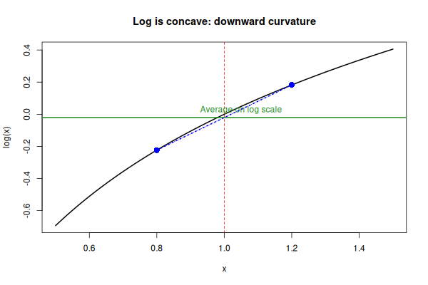
The Intuition First (No Math): You have a tumor volume \(T = 1.0\). Over a tiny time step, you add random noise that is symmetric on the original scale:
- 50% chance of multiplying by \(1.2\) (up 20%)
- 50% chance of multiplying by \(0.8\) (down 20%)
What is the average outcome?
- Arithmetic mean = \((1.2 + 0.8)/2 = \mathbf{1.0}\) (no net change)
At the log scale:
- Log up: \(\log(1.2) = 0.182\)
- Log down: \(\log(0.8) = -0.223\)
- Arithmetic mean on log scale = \((0.182 - 0.223)/2 = \mathbf{-0.0205}\)
The average log is negative even though the average original volume is 1.0!
That \(-0.0205\) is approximately \(-\sigma^2/2\) (here \(\sigma \approx 0.2\), the step-wise change).
This is because log is concave (it curves downward): When you take a symmetric step on the original scale (multiply by \(1+\delta\) or \(1-\delta\)), the log of the downward step is more negative than the log of the upward step is positive. This creates a negative bias on the log scale.
The Mathematical Derivation (Itô’s Lemma)
SDE on original scale:
\[dT = \lambda T dt + \sigma T dW\]
if we assume \(x = \log T\)
Itô’s lemma says: for \(x = g(T)\), \[dx = \frac{\partial x}{\partial T} dT + \frac12 \frac{\partial^2 x}{\partial T^2} (dT)^2\]
or:
\[dx = g'(T) dT + \frac{1}{2} g''(T) (dT)^2\]
Where \(g(T) = \log T\), \(g'(T) = 1/T\), and \(g''(T) = -1/T^2\).
The key rule of stochastic calculus: \((dW)^2 = dt\), and cross terms \(dt \cdot dW = 0\).
So: \[(dT)^2 = (\lambda T dt + \sigma T dW)^2 = \sigma^2 T^2 (dW)^2 = \sigma^2 T^2 dt\]
Plug into Itô’s lemma: \[dx = \frac{1}{T} (\lambda T dt + \sigma T dW) + \frac{1}{2} \left(-\frac{1}{T^2}\right) (\sigma^2 T^2 dt)\]
Simplify each term:
- First term: \(\frac{1}{T} \cdot \lambda T dt = \lambda dt\)
- Second term: \(\frac{1}{T} \cdot \sigma T dW = \sigma dW\)
- Third term: \(\frac{1}{2} \cdot (-\frac{1}{T^2}) \cdot \sigma^2 T^2 dt = -\frac{1}{2} \sigma^2 dt\)
Add them up: \[dx = \lambda dt + \sigma dW - \frac{1}{2} \sigma^2 dt\]
\[dx = \left(\lambda - \frac{\sigma^2}{2}\right) dt + \sigma dW\]
That’s where \(-\sigma^2/2\) comes from. It is from the \((dT)^2\) term that contains \((dW)^2 = dt\), producing this famous \(-\sigma^2/2\) correction.