Understanding Gaussian Process: A Foundation

statistics

bayesian statistics

gaussian process

probability

inference

advanced

Published

September 3, 2026

If you’ve ever wanted to put smooth curves through noisy data and get honest uncertainty estimates along the way, a Gaussian Process (GP) is the best choice. Intuitively, GP is a probability distribution over functions. Instead of giving you a single best‑fit curve, a GP places a probability distribution over the whole space of functions that could explain your data. Hence, a GP can also be considered as a distribution of possible curves that are consistent with your data, complete with uncertainty estimates.

The formal definition

A Gaussian Process is:

A collection of random variables, any finite subset of which is jointly Gaussian.

Let’s translate that word by word.

“A collection of random variables”
A function \(f\) can be thought of as an infinite collection of random variables: one for each possible input \(x\). We label them \(f(x_1), f(x_2), f(x_3), \dots\). There are uncountably many of them if \(x\) is continuous, but we don’t need to list them all. The GP is this entire collection.

“Any finite subset of which is jointly Gaussian”
You cannot directly handle an infinite-dimensional Gaussian distribution. So instead, the definition makes a promise: no matter which finite set of input points you choose to look at, the corresponding function values will follow a standard multivariate Gaussian distribution. Pick 5 points? Jointly Gaussian. Pick 10,000 points? Jointly Gaussian. Every possible finite slice of the process is a familiar Gaussian distribution you can work with.

This is what allows us to do all the practical computations with finite matrices—while the underlying object remains an infinite-dimensional distribution over functions.

The Two-Layer Summary of a Gaussian Process

Layer	What it is
Conceptual	A probability distribution over an infinite-dimensional space of functions.
Operational	A rule saying: for any finite set of inputs, the outputs follow a multivariate Gaussian with mean \(m\) and covariance \(k\).

The operational layer is how we define and compute with the conceptual layer, sidestepping the need to ever manipulate infinite-dimensional objects directly.

The prior: before seeing any data

A GP is fully and uniquely defined by two things:

A mean function \(m(x)\) — the expected function value at input \(x\).
\(m(x) = \mathbb{E}[f(x)]\)
A covariance function (kernel) \(k(x, x')\) — how any two function values \(f(x)\) and \(f(x')\) co-vary.
\(k(x, x') = \text{Cov}[f(x), f(x')]\)

We write: \[ f(x) \sim \mathcal{GP}(m(x), k(x, x')) \]

For most practical work we take \(m(x)=0\) after centering the data, so the kernel does all the heavy lifting.

Before observing any data, the GP defines a prior over functions. For any finite set of inputs, the function values follow:

\[p(\mathbf{f}) = \mathcal{N}(\mathbf{0}, K)\]

where \(K_{ij} = k(x_i, x_j)\).

This prior encodes our assumptions about smoothness, periodicity, amplitude, and other properties through the choice of kernel.

What parameters define a kernel?

Most kernels have a small number of hyperparameters that control the shape of the functions we expect. The most common ones are:

Signal Variance (\(\sigma^2\))

This controls the vertical scale or amplitude of the function. It determines how far the function is expected to deviate from its mean. A larger value means the function can take on larger values overall.

Lengthscale (\(\ell\) or \(\rho\))

This controls the horizontal scale, or how quickly the function changes with respect to the input, or how fast the correlation decays with distance in \(x\). It determines the “wiggliness” of the functions:
- Short lengthscale: The function can vary rapidly (high frequency), capturing fine details.
- Long lengthscale: The function is very smooth (low frequency), capturing only broad trends.

Noise Variance (\(\sigma^2_{n}\))

This is often added to the diagonal of the covariance matrix to account for observation noise or numerical stability. It represents the amount of unexplained variance in the data.

Common Kernels

The kernel is the heart of a GP. It encodes your assumptions about the function you’re trying to model. Here are the most common choices:

Squared Exponential (SE) / RBF Kernel

\[ k_{\text{SE}}(x, x') = \sigma^2 \exp\left(-\frac{(x - x')^2}{2\ell^2}\right) \]

This is the “default” kernel. It assumes the function is infinitely smooth (infinitely differentiable) and that points closer together are more strongly correlated. The lengthscale determines how quickly this correlation decays. This kernel is a stationary kernel, meaning the covariance depends only on the distance \(|x - x'|\) and not on the absolute location of \(x\) or \(x'\). Therefore, shifting both input points by the same amount does not change their covariance.

Use when: You expect the underlying function to be very smooth and continuous.

Matérn Kernel

\[ k_{\mathrm{Matérn32}}(r) = \sigma^2\left(1 + \frac{\sqrt{3}r}{\ell}\right)\exp\!\left(-\frac{\sqrt{3}r}{\ell}\right), \quad r = |x-x'|. \]

A flexible family that can model rougher functions. The Matérn 3/2 (as shown above. It is \(\nu=3/2\) in generalised form) and 5/2 are popular choices when you don’t want the extreme smoothness of the RBF kernel. This is another stational kernel.

Use when: You want more control over smoothness or have reason to believe the function is not infinitely smooth.

Unfold to see the general form

For completeness, the general Matérn kernel for any \(\nu > 0\) is: \[ k_{\text{Matérn}}(r) = \sigma^2 \frac{2^{1-\nu}}{\Gamma(\nu)} \left(\frac{\sqrt{2\nu} \cdot r}{\ell}\right)^{\nu} K_{\nu}\left(\frac{\sqrt{2\nu} \cdot r}{\ell}\right) \]

Where \(K_\nu\) is a modified Bessel function. The 3/2 and 5/2 cases above are what you get when \(\nu\) is a half-integer and the Bessel function simplifies.

This is a generalization of the SE kernel. It has an extra parameter \(\nu\) that controls the smoothness of the function:

\(\nu = 1/2\): Functions are not differentiable (rough).
\(\nu = 3/2\): Functions are once differentiable.
\(\nu = 5/2\): Functions are twice differentiable.
\(\nu \to \infty\): Converges to the SE kernel.

Rational Quadratic (RQ) Kernel

\[ k_{\text{RQ}}(x, x') = \sigma^2 \left(1 + \frac{(x - x')^2}{2\alpha \ell^2}\right)^{-\alpha} \]

This kernel is equivalent to a sum of many SE kernels with different lengthscales. It captures variation at multiple scales. \(\alpha\) is a positive shape/mixture parameter that controls the relative weighting of large-scale vs small-scale variations. As \(\alpha\) increases, the RQ kernel approaches the SE kernel, whereas smaller \(\alpha\) allows for more long-range correlations. As SE and Matérn kernels, the RQ kernel is also stationary.

Use when: You expect the function to have both short-term and long-term patterns.

Periodic Kernel

\[ k_{\text{Periodic}}(x, x') = \sigma^2 \exp\left(-\frac{2\sin^2(\pi|x - x'|/p)}{\ell^2}\right) \]

This kernel is designed to model periodic functions. It has an extra parameter \(p\) that controls the period. This is also a stationary kernel, as the covariance depends only on the distance \(|x - x'|\) and not on the absolute location of \(x\) or \(x'\).

Use when: You expect the function to have repeating patterns.

Linear kernel

\(k(x,x') = \sigma_b^2 + \sigma_v^2\, x x'\)

Useful for Bayesian linear regression:

\(\sigma_b^2\) — the bias (or offset) variance. It controls how far the regression line can be from zero at \(x = 0\). If you set this to zero, all functions are forced to pass through the origin.
\(\sigma_v^2\) — the slope (or linear coefficient) variance. It controls how steep the lines can be. A large \(\sigma_v^2\) gives widely varying slopes.
no lengthscale — The linear kernel is non-stationary—its covariance grows as \(|x|\) and \(|x'|\) grow (hence depends on absolute positions). It doesn’t have the “nearby points are more correlated” property that a lengthscale encodes.

A linear kernel defines a distribution over straight lines (or hyperplanes in higher dimensions), with no local wiggliness. It’s equivalent to Bayesian linear regression with Gaussian priors on the weights.

White noise kernel

\[ k_{\text{white}}(x, x') = \sigma_n^2 \cdot \delta(x, x') \]

where \(\delta(x, x')\) is 1 if \(x = x'\) and 0 otherwise. In practice, this adds a diagonal term \(\sigma_n^2 I\) to your covariance matrix.

You can add it directly to another kernel:

\[ k_{\text{total}} = k_{\text{RBF}} + k_{\text{white}} \]

The white noise kernel models i.i.d. observation noise (i.i.d. stands for independent and identically distributed)—the random measurement error that makes your observed \(y\) differ from the true underlying \(f(x)\). This means the noise is part of your GP prior. The covariance matrix becomes \(K + \sigma_n^2 I\) naturally.

Alternatively, you can add noise via the likelihood:

\[ y = f(x) + \epsilon, \quad \epsilon \sim \mathcal{N}(0, \sigma_n^2) \]

Then \(f \sim \mathcal{GP}(0, k)\) and you add \(\sigma_n^2 I\) when computing the posterior. This is the more common formulation in modern GP libraries (GPy, GPflow, scikit-learn’s alpha parameter).

Please note that the white noise kernel add variance to the diagonal of the covariance matrix, which add independent measurement error that does not propogate to off-diagonal elements which is the covariance between different points. To properly change the signal variance in a kernel, you need to change the variance parameter of the kernel itself (e.g., \(\sigma^2\) in RBF or Matérn), or multiply the kernel by a constant.

Combining Kernels

You can add or multiply kernels to create more complex structures. For example, adding a periodic kernel to an SE kernel can model a function that has a seasonal pattern with an overall trend.

Sum: \(k = k_1 + k_2\) is valid if both are valid.
Product: \(k = k_1 \times k_2\) is valid if both are valid.
Scaling: \(k = c \cdot k_1\) is valid for \(c > 0\).
Exponentiation: \(k = \exp(k_1)\) is valid if \(k_1\) is a valid kernel (with some caveats—this is the basis of the RBF kernel derived from the squared-exponential of the linear kernel).

What makes a valid kernel?

A kernel is valid if and only if, for any set of points you could ever choose, the resulting covariance matrix has no negative eigenvalues. This ensures every variance is positive and every uncertainty is meaningful. If a kernel produced a negative eigenvalue, the mathematics of Gaussian distributions would break down—you’d get negative probabilities.

That is, for any vectors \(x_1, \dots, x_N\) and any coefficients \(c_1, \dots, c_N\):

\[ \sum_{i=1}^N \sum_{j=1}^N c_i c_j \, k(x_i, x_j) \geq 0 \]

The prior distribution of common kernels

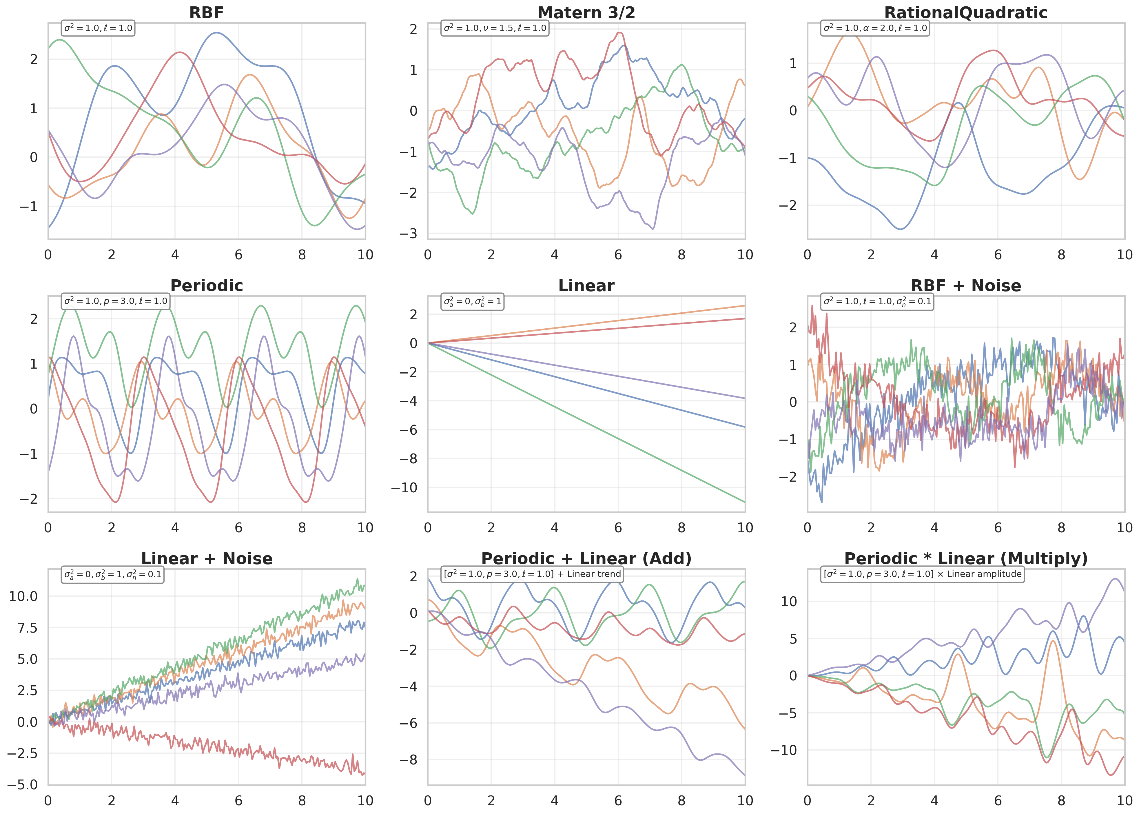
Unfold to see the python code for kernel definition

import numpy as np
import matplotlib.pyplot as plt
import seaborn as sns
from sklearn.gaussian_process.kernels import (RBF, Matern, RationalQuadratic, 
                                              ExpSineSquared, DotProduct,WhiteKernel,ConstantKernel)

# Set seaborn style
sns.set_theme(style="whitegrid", context="talk")

## Input x and set up kernel
# --- 1. Settings ---
x = np.linspace(0, 10, 200).reshape(-1, 1)
length_scale = 1.0
variance = 1.0               # Global signal variance (σ²)
intercept_variance = 0     # For linear kernel intercept
slope_variance = 1         # For linear kernel slope

# --- 2. Kernel Configurations (Variance is defined INSIDE each kernel by multiplying a constant) ---
# Please note: 
#   kerneals in sklearn gaussian_process only defines the correlation part (the exponent part), not the variance. 
#   The variance need to be defined by multiplying the kernal output with a constant, representing the variance. 
#   WhiteKernel output need to be derived by kernal_instal(x), other than kernal_instance(x,x), so you can NOT define a new kernel by adding whitenoise kernel at the class definition level
kernel_configs = {
    "RBF": {
        "kernel": ConstantKernel(variance) * RBF(length_scale=length_scale),
        "noise": 0.0,
        "params": rf"$\sigma^2 = {variance}, \ell = {length_scale}$"
    },
    "Matern 3/2": {
        # mertan 32, nu=1.5, mertan 52, nu=2.5
        "kernel": ConstantKernel(variance) * Matern(length_scale=length_scale, nu=1.5),
        "noise": 0.0,
        "params": rf"$\sigma^2 = {variance}, \nu = 1.5, \ell = {length_scale}$"
    },
    "RationalQuadratic": {
        "kernel": ConstantKernel(variance) * RationalQuadratic(length_scale=length_scale, alpha=2.0),
        "noise": 0.0,
        "params": rf"$\sigma^2 = {variance}, \alpha = 2.0, \ell = {length_scale}$"
    },
    "Periodic": {
        "kernel": ConstantKernel(variance) * ExpSineSquared(length_scale=length_scale, periodicity=3.0),
        "noise": 0.0,
        "params": rf"$\sigma^2 = {variance}, p = 3.0, \ell = {length_scale}$"
    },
    "Linear": {
        # DotProduct kernel = sigma_0^2 + x^T x', where sigma_0^2 is the intercept variance, here we define it to be 0 in order to define both intercept and slope variance separately
        "kernel": ConstantKernel(intercept_variance) + ConstantKernel(slope_variance) * DotProduct(sigma_0=0),
        "noise": 0.0,
        "params": rf"$\sigma_a^2={intercept_variance}, \sigma_b^2={slope_variance}$"
    },
    "RBF + Noise": {
        "kernel": ConstantKernel(variance) * RBF(length_scale=length_scale),
        "noise": 0.1,
        "params": rf"$\sigma^2 = {variance}, \ell={length_scale}, \sigma_n^2=0.1$"
    },
    "Linear + Noise": {
        "kernel": ConstantKernel(intercept_variance) + ConstantKernel(slope_variance) * DotProduct(sigma_0=0),
        "noise": 0.1,
        "params": rf"$\sigma_a^2={intercept_variance}, \sigma_b^2={slope_variance}, \sigma_n^2=0.1$"
    },
    "Periodic + Linear (Add)": {
        # this will give a straight line upwards trend but with oscilation on top
        "kernel": ConstantKernel(variance) * ExpSineSquared(length_scale=length_scale, periodicity=3.0) 
                  + ConstantKernel(intercept_variance) + ConstantKernel(slope_variance) * DotProduct(sigma_0=0),
        "noise": 0.0,
        "params": rf"[$\sigma^2={variance}, p=3.0, \ell={length_scale}$] + Linear trend"
    },
    "Periodic * Linear (Multiply)": {
        # amplitude of the periodic function will increase linearly with x, which is a common pattern in many real-world time series data
        "kernel": ConstantKernel(variance) * ExpSineSquared(length_scale=length_scale, periodicity=3.0) 
                  * (ConstantKernel(intercept_variance) + ConstantKernel(slope_variance) * DotProduct(sigma_0=0)),
        "noise": 0.0,
        "params": rf"[$\sigma^2={variance}, p=3.0, \ell={length_scale}$] $\times$ Linear amplitude"
    }
}

# --- 3. Create the grid ---
fig, axes = plt.subplots(3,3, figsize=(20, 14))
axes = axes.flatten()
# fig.delaxes(axes[-1])  # Remove the extra empty subplot

# --- 4. Plot each kernel ---
n_samples = 5

for ax, (name, config) in zip(axes, kernel_configs.items()):
    kernel = config["kernel"]
    
    # --- Variance is already inside the kernel! ---
    # No need to multiply by variance here.
    # However, noise is not yet defined in the kernel.
    K = kernel(x, x)
    if config["noise"] > 0:
        K += WhiteKernel(noise_level=config["noise"])(x)
    
    # Sample 5 functions from the prior
    y_samples = np.random.multivariate_normal(mean=np.zeros(len(x)), cov=K, size=n_samples).T
    
    # Plot the sampled functions
    for i in range(n_samples):
        ax.plot(x, y_samples[:, i], alpha=0.7, lw=2)
    
    
    ax.set_title(name, fontsize=14, fontweight='bold')
    ax.grid(True, alpha=0.3)
    ax.set_xlim(0, 10)

    # --- Parameter annotation inside the plot in a box with a fox ---
    ax.text(0.05, 1.0, config["params"], transform=ax.transAxes, fontsize=11,
            verticalalignment='top',
            bbox=dict(boxstyle='round,pad=0.3', facecolor='white', edgecolor='gray', alpha=0.9))

# Adjust layout to prevent clipping
plt.tight_layout(rect=[0, 0.15, 1, 0.95])

plt.show()

How to choose a kernel

Choosing a kernel is part art, part science. Here are some guiding principles:

Smoothness – If you expect your function to be very smooth, start with an RBF or Matern 5/2. For rougher functions, try Matern 3/2 or 1/2.
Stationarity – Most standard kernels are stationary (depend only on distance: \(x - x'\), such as RBF and Matérn). If your data have a clear trend, you might combine a stationary kernel with a linear mean function.
Periodicity – If the data show cycles, include a periodic kernel, possibly multiplied by a local RBF to allow the periodic pattern to change over time.
Additive structure – Sums of kernels correspond to sums of independent functions. For example, a smooth trend plus a periodic component: \(k = k_{\mathrm{RBF}} + k_{\mathrm{Per}}\).
Automatic relevance determination (ARD) – For multidimensional inputs, you can give each input dimension its own lengthscale, so the model can “turn off” irrelevant dimensions.
Model selection – You can use the marginal likelihood (the “evidence”) to compare different kernels and optimise hyperparameters. The marginal likelihood automatically trades off fit and complexity.

A good practical strategy: start simple with an RBF kernel and optimise the lengthscale and variance. Then inspect the residuals and increase complexity only if the data demand it.

Do GPs have knots or nodes?

This is a common point of confusion. Standard Gaussian processes do not have knots or nodes. The whole idea of a GP is that it defines a distribution directly over functions, without discretising the input space with basis functions or splines.

In spline methods, “knots” are fixed locations where the basis functions meet, and you place a coefficient at each knot.
In some sparse Gaussian process approximations, you introduce a set of inducing points (often also called “pseudo‑inputs” or “inducing inputs”). These are a small number of locations \(Z = \{z_1, \dots, z_M\}\) that summarise the full dataset, making computations \(O(N M^2)\) instead of \(O(N^3)\).
Those inducing points are learned parameters; they are not part of the standard full GP story.

So if you hear “knots” in the context of GPs, it’s almost always about sparse approximations. For our basic understanding, just remember: a full GP has no knots – it is a non‑parametric model that uses the whole dataset as “basis” points. Every data point is essentially a new “feature”.

The posterior: what the GP believes after seeing data

When you receive data \(\mathcal{D} = \{(\mathbf{x}_i, y_i)\}_{i=1}^N\), the prior GP is updated to a posterior GP in one single step.

The prior: \(f \sim \mathcal{GP}(0, k)\), or \(p(\mathbf{f}) = \mathcal{N}(\mathbf{f} \mid \mathbf{0}, K)\)
The likelihood: \(p(\mathbf{y} \mid \mathbf{f}) = \mathcal{N}(\mathbf{y} \mid \mathbf{f}, \sigma_n^2 I)\)
The posterior: \(f \mid \mathbf{y} \sim \mathcal{GP}(m_{\text{post}}, k_{\text{post}})\), or \(p(\mathbf{f} \mid \mathbf{y})\)

Bayes’ theorem gives the posterior over the latent function values at the observed inputs:

\[p(\mathbf{f} \mid \mathbf{y}) = \frac{\mathcal{N}(\mathbf{y} \mid \mathbf{f}, \sigma_n^2 I) \, \mathcal{N}(\mathbf{f} \mid \mathbf{0}, K)}{p(\mathbf{y})} = \mathcal{N}\big(\mathbf{f} \mid K(K+\sigma_n^2 I)^{-1}\mathbf{y},\; K - K(K+\sigma_n^2 I)^{-1}K\big)\]

Please read this post for the full derivation of posterior GP and how new inputs are predicted.

Fitting to synthetic time‑course data

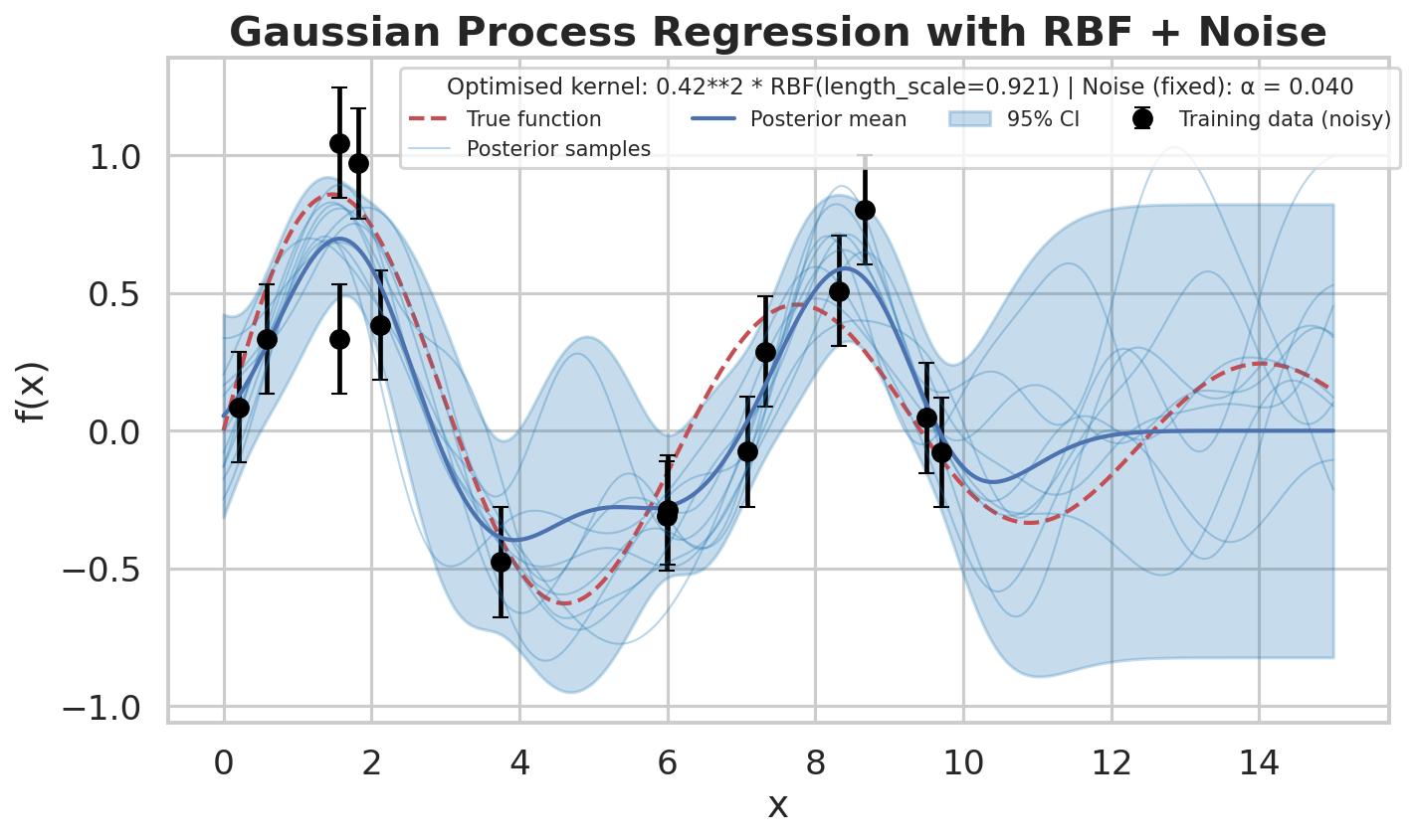
To illustrate how a Gaussian Process (GP) performs regression in practice, we generated a small synthetic dataset with 15 noisy observations from a damped sine wave:

\[ f(x) = \sin(x) \cdot e^{-0.1x} \]

We added independent Gaussian noise with a standard deviation of \(0.2\) to simulate real-world measurement errors.

For the GP model, we chose a squared exponential (RBF) kernel to encode the prior belief that the underlying function is smooth.

We did not fix the kernel hyperparameters (\(\ell\) and \(\sigma^2\)) in advance. Instead, we let the model learn them from the data by maximising the log-marginal-likelihood (as we used Scikit-learn, the hyperparameters are not inferred by Bayesian methods). The noise variance was fixed to the true value used to generate the data (\(0.2^2 = 0.04\)) to keep the demonstration clean.

Unfold to see the python code for GP regression

import numpy as np
import matplotlib.pyplot as plt
import seaborn as sns
from sklearn.gaussian_process import GaussianProcessRegressor
from sklearn.gaussian_process.kernels import ConstantKernel, RBF

# --- 1. Apply Seaborn styling globally ---
sns.set_theme(style="whitegrid", context="talk")  # 'talk' gives nice large fonts

# --- 2. Generate synthetic data with noise---
np.random.seed(42)
x_train = np.sort(np.random.uniform(0, 10, 15)).reshape(-1, 1)
true_f = lambda x: np.sin(x) * np.exp(-0.1 * x)
y_train = true_f(x_train).ravel() + 0.2 * np.random.randn(len(x_train))

x_test = np.linspace(0, 15, 300).reshape(-1, 1)

# --- 3. Define the kernel with bounds ---
kernel = ConstantKernel(1.0, constant_value_bounds=(1e-3, 1e3)) * RBF(
    length_scale=1.0, length_scale_bounds=(1e-2, 1e2)
)

# --- 4. Fit the GP (noise variance fixed to 0.04) ---
# the fact that alpha is adding noise is verified by GP posterior curves are not deliberately going through all training points, but rather "smoothing" around them.
gp = GaussianProcessRegressor(
    kernel=kernel, 
    alpha=0.2**2,              # noise variance = 0.04
    n_restarts_optimizer=10,
    random_state=42
)
gp.fit(x_train, y_train)

# --- 5. Predict on test points ---
# mean equals median for Gaussian distribution, and std is the uncertainty
y_mean, y_std = gp.predict(x_test, return_std=True)

# --- Sample 10 functions from the posterior ---
y_samples = gp.sample_y(x_test, n_samples=10, random_state=42)

# --- Print the learned hyperparameters ---
print("Learned kernel:", gp.kernel_)

Notice how the uncertainty shrinks near the training points (where data is available) and widens in regions with no data (e.g., between observations and at the edges of the domain).

Wrapping up and Nuances with Scikit-learn

Gaussian Processes (GPs) are a powerful class of non‑parametric Bayesian methods. Rather than assuming a fixed parametric form for the underlying function, a GP places a prior directly over the space of functions via a kernel (covariance function), and then updates this prior to a posterior given observed data. Their core strengths are:

Non‑parametric nature: The complexity of the model grows with the data, avoiding the need to pre‑specify the number of basis functions or polynomial degree.
No fixed “knobs”: While the kernel has hyperparameters (e.g., length scale, signal variance), these can be learned from the data, meaning the model adapts to the complexity of the problem at hand.
Principled uncertainty quantification: Every prediction comes with a full posterior distribution—not just a point estimate. This provides credible intervals that are wider where data is sparse and narrower near observations.
Finite data, infinite functions: By defining a multivariate Gaussian distribution over a finite set of observed and test points, the GP infers a distribution over the continuous, infinite‑dimensional function space.

When implementing GP regression with scikit-learn’s GaussianProcessRegressor, there are several important practical nuances to be aware of:

Kernel definition: The built‑in RBF kernel (and similar ones) in scikit-learn defines only the correlation (exponential) part. By default, it does not include the signal variance \(\sigma^2\). To incorporate the signal variance, you must explicitly multiply it by a ConstantKernel, e.g., ConstantKernel(sigma_squared) * RBF(length_scale).
The WhiteKernel caveat: Unlike most kernels where kernel(X, X) returns the full covariance matrix, WhiteKernel behaves differently. Calling WhiteKernel(X, X) returns a zero matrix, whereas WhiteKernel(X) returns the correct diagonal noise matrix. This means combining WhiteKernel with other kernels using the standard kernel(X, X) call will silently drop the noise term—making the combination cumbersome. To correctly build the covariance matrix for plotting or custom sampling, you must explicitly separate the components: K = base_kernel(X, X) + WhiteKernel(X).
Noise handling in GaussianProcessRegressor: For fitting a GP regression model, the officially recommended way to handle independent Gaussian measurement noise is not via WhiteKernel, but by using the alpha parameter. alpha directly adds the noise variance to the diagonal of the kernel matrix during training, which is simpler, more robust, and avoids the WhiteKernel pitfall entirely.
Hyperparameter optimisation: By default, scikit-learn learns the kernel hyperparameters (length scale, signal variance, etc.) by maximising the log‑marginal‑likelihood (MLE). You can set bounds on these parameters to restrict the search space, but you cannot specify a prior distribution over them, nor does the implementation perform full Bayesian inference over the hyperparameters. This yields a point estimate of the hyperparameters, meaning the uncertainty associated with the hyperparameter estimates themselves is not propagated into the final predictions. Another practical nuance is that the noise variance can be optimised (point estimate) alongside the other hyperparameters—but only if you explicitly include a WhiteKernel in the kernel definition (however, be careful about how to incorporate it as stated in point 2). If you use the alpha parameter to fix the noise (as in above example), that value is not optimised during fitting; it remains constant.
Posterior vs. MCMC: GaussianProcessRegressor does not rely on MCMC sampling for the posterior distribution. For standard regression with a Gaussian likelihood, the posterior is analytically tractable (via closed‑form matrix algebra), which makes it computationally efficient for moderate‑sized datasets. This analytical approach is the core reason for scikit-learn’s computational speed, but it also means that the hyperparameter optimisation step itself remains a deterministic point‑estimate.