Beginner’s guide to Bayesian Statistics: Prior, Likelihood, and Posterior

In the previous post, we introduced the core mechanics of Bayesian statistics: the Bayes’ theorem through two striking examples — Steve the librarian and the rare disease screening test. We saw how ignoring the prior knowledge can lead us astray, and we learned to combine prior knowledge with observed data using the Bayes’ theorem:

\[ P(H|D) = \frac{P(H) \cdot P(D|H)}{P(D)} \]

We then took our first step beyond point estimates. Instead of treating the disease prevalence and screening sensitivity as single fixed numbers, we expressed our uncertainty about them via distributions:

\[ \begin{aligned} \text{Sick} &\sim \text{Beta}(1, 9999) \\ P(\text{Positive}|\text{Sick}) &\sim \text{Beta}(999, 1) \end{aligned} \]

We assembled these into a simplified Bayesian model assuming the false positive rate \(\beta = P(\text{Positive}|\text{No Sick})\) as a known constant, typically from the test manufacturer’s specifications.

\[ P(\text{Sick} | \text{Positive}) = \frac{P(\text{Sick}) \cdot P(\text{Positive}|\text{Sick})}{\int P(\text{Sick}) \cdot P(\text{Positive}|\text{Sick}) \, dP(\text{Sick})} \]

Now we’re going to take this example further

In reality, we’re not completely certain about the false positive rate either. It comes from the same validation studies as the sensitivity, with the same limited sample sizes. So in this post, we’ll build a full Bayesian model that treats all three quantities as uncertain:

• Prevalence: \(\theta = P(\text{Sick})\) — the true disease rate in the population.
• Sensitivity: \(\alpha = P(\text{Positive}|\text{Sick})\) — the probability of testing positive if sick.
• False Positive Rate: \(\beta = P(\text{Positive}|\text{No Sick})\) — the probability of testing positive if healthy. Specificity, \(\gamma = 1 - \beta\).

Each gets its own prior distribution. The likelihood becomes more complex because the observed positives come from two sources: sick people who test positive (true positives) and healthy people who test positive (false positives). The posterior becomes a joint distribution over all three parameters. And the marginal likelihood (the denominator) becomes a triple integral that typically requires computational methods like MCMC.

And finally, for the observations:

• \(N\) = total number of people tested.
  
• \(\text{Positive}\) = total number of positive test results.

We do not know exactly who are really sick or healthy. However, this observation allows us to infer and update the posterior distributions of \(\theta\), \(\alpha\), and \(\beta\), and ultimately compute the posterior predictive distribution for a new individual who tests positive.

---

Priors as Distributions

Each parameter is assumed to be a random draw from a distribution with its “location” and “scale” defined by distribution-specific parameters. This type of distribution is called the prior distribution representing our prior beliefs about the rare disease, and highly sensitive and specific screening before seeing the data.

We define priors for the three parameters with beta distributions, which defines the probabilities of having different values for the success probability ([0,1]) of a Bernoulli trial. The first value in a beta distribution represents the number of successes, and the second value represents the number of failures. The higher both values, the more confident we are about the mean of the distribution.

\[ \begin{aligned} \theta &\sim \text{Beta}(1, 9999) \, \text{(prevalence: rare disease, mean = 0.0001)} \\ \alpha &\sim \text{Beta}(999, 1) \, \text{(sensitivity: highly sensitive test, mean = 0.999)} \\ \beta &\sim \text{Beta}(1, 999) \, \text{(false positive rate: highly specific test, mean = 0.001)} \end{aligned} \]

---

Priors Come in Flavours

Not all priors are created equal. Here are the common types:

1. Informative priors — based on real data or strong expert knowledge. Use these when you actually know something.

In our disease example, \(\alpha \sim \text{Beta}(999, 1)\) is an informative prior for sensitivity — it expresses a strong belief that the test is around 99.9% accurate. However, it is less confident than a prior like \(\text{Beta}(999000, 1000)\), even though both have the same mean. The latter would be based on a much larger validation study, and would be more confident about the mean and “harder” to be overturned by new data. The stronger the prior, the more data it takes to override it.

2. Weak (or diffuse) priors — like \(\text{Beta}(9, 1)\). They say “I have a slight inclination, but the data can easily override me.” These are useful when you have some idea but don’t want to force your belief onto the results.

3. “Uninformative” priors — like \(\text{Beta}(1, 1)\) (the uniform distribution, “everything is equally possible”) or \(\text{Beta}(0, 0)\) (the Haldane prior, “everything is impossible”).

But here’s the controversial take: there’s no such thing as a truly “fair” prior. When you know absolutely nothing, it’s better to admit you can’t conclude anything than to use a prior that is so uninformative it might produce unrealistic results.

A note of caution: As data accumulates, the posterior distribution converges toward the likelihood — the data “speaks for itself” regardless of your prior (unless your prior is extremely strong). So don’t lose sleep over choosing the “perfect” prior. Pick something reasonable, exclude the impossible values, and let the data do the talking.

---

Likelihood: What the Data Says

The likelihood \(P(\text{Positive} | \theta, \alpha, \beta)\) is the probabilities of observing your data given your hypothesis (parameter values). In our disease example, the data is the total number of positive tests.

The probability that a randomly selected individual tests positive is:

\[ p_{\text{pos}} = \alpha \cdot \theta + \beta \cdot (1 - \theta) \]

Because:
- With probability \(\theta\), the person is sick and tests positive with probability \(\alpha\).
- With probability \(1 - \theta\), the person is healthy and tests positive with probability \(\beta\).

Therefore, the total number of positive tests follows a Binomial distribution:

\[ \text{Positive} \sim \text{Binomial}(N, \, \alpha \cdot \theta + \beta \cdot (1 - \theta)) \]

This is the likelihood: it tells us how probable the observed number of positive tests is, for any given combination of prevalence, sensitivity, and false positive rate.

For the mathematically curious: If we observed individual test results rather than just the total, the likelihood would be a product over each person’s result — positive or negative — with probabilities \(\alpha \cdot \theta + \beta \cdot (1 - \theta)\) for positive and the complement for negative. The Binomial distribution is just the compressed version.

Unfold to see the full derivation from the full likelihood to the above simplified one

The Full Likelihood: From First Principles

To construct the likelihood from first principles, imagine we tested \(N\) people and observed exactly \(p\) positive results. We don’t know which individuals are sick or healthy, nor do we know how many of the positive results came from sick versus healthy people. The data-generating process has three layers of randomness: first, the number of sick people \(S\) is drawn from a Binomial distribution based on the prevalence \(\theta\); second, among those \(S\) sick people, the number of true positives \(TP\) follows a Binomial distribution with sensitivity \(\alpha\); third, among the remaining \(N - S\) healthy people, the number of false positives \(FP\) follows a Binomial distribution with false positive rate \(\beta\). The total observed positives are the sum \(p = TP + FP\). Since we observe neither \(S\), \(TP\), nor \(FP\), the full likelihood is obtained by summing over all possible combinations of these unobserved quantities that are consistent with the observed total \(p\):

\[ \begin{aligned} P(\text{Positive} = p \mid \theta, \alpha, \beta) = \sum_{S=0}^{N} \, \sum_{TP=0}^{S} \, \sum_{FP=0}^{N-S} &\left[ \binom{N}{S} \theta^{S} (1-\theta)^{N-S} \right] \\[4pt] &\times \left[ \binom{S}{TP} \alpha^{TP} (1-\alpha)^{S-TP} \right] \\[4pt] &\times \left[ \binom{N-S}{FP} \beta^{FP} (1-\beta)^{N-S-FP} \right] \\[4pt] &\times \mathbf{1}(TP + FP = p). \end{aligned} \]

Indicator function:
The term \(\mathbf{1}(TP + FP = p)\) ensures that we only sum over combinations of true positives and false positives whose total exactly equals the observed number of positive tests \(p\).

Multiplication in the likelihood:
We multiply the three Binomial probabilities because the number of sick individuals \(S\), the true positives among them \(TP\), and the false positives among the healthy \(FP\) arise from sequential, conditionally independent processes — first the population is split into sick and healthy, then each subgroup independently produces its own positive counts — so their joint probability is the product of their individual probabilities.

Rewrite the Full Likelihood

The full likelihood can be written more compactly by combining the three Binomial terms:

\[ P(\text{Positive} = p \mid \theta, \alpha, \beta) = \sum_{S=0}^{N} \sum_{TP=0}^{S} \sum_{FP=0}^{N-S} \frac{N!}{S!(N-S)!} \theta^{S} (1-\theta)^{N-S} \cdot \frac{S!}{TP!(S-TP)!} \alpha^{TP} (1-\alpha)^{S-TP} \cdot \frac{(N-S)!}{FP!(N-S-FP)!} \beta^{FP} (1-\beta)^{N-S-FP} \cdot \mathbf{1}(TP + FP = p). \]

Cancel Common Factorials

Notice that \(S!\) and \((N-S)!\) cancel between the terms:

\[ P(\text{Positive} = p \mid \theta, \alpha, \beta) = \sum_{S=0}^{N} \sum_{TP=0}^{S} \sum_{FP=0}^{N-S} \frac{N!}{TP! \, FP! \, (S-TP)! \, (N-S-FP)!} \cdot \theta^{S} (1-\theta)^{N-S} \cdot \alpha^{TP} (1-\alpha)^{S-TP} \cdot \beta^{FP} (1-\beta)^{N-S-FP} \cdot \mathbf{1}(TP + FP = p). \]

Reorganize the Exponents

We can rearrange the powers to group terms by whether a person is sick/healthy and positive/negative. Notice that:

• \(\theta^{S} = \theta^{TP + (S-TP)} = \theta^{TP} \cdot \theta^{S-TP}\)
• \((1-\theta)^{N-S} = (1-\theta)^{FP + (N-S-FP)} = (1-\theta)^{FP} \cdot (1-\theta)^{N-S-FP}\)

So the full expression becomes:

\[ P(\text{Positive} = p \mid \theta, \alpha, \beta) = \sum_{\substack{S, TP, FP \\ TP + FP = p}} \frac{N!}{TP! \, FP! \, (S-TP)! \, (N-S-FP)!} \cdot (\theta \alpha)^{TP} \cdot (\theta (1-\alpha))^{S-TP} \cdot ((1-\theta) \beta)^{FP} \cdot ((1-\theta)(1-\beta))^{N-S-FP}. \]

Factor Out the Observed Categories

Notice that the terms involving \(TP\) and \(FP\) (the positive categories) are “fixed” by the observation \(p = TP + FP\). The terms involving \(S-TP\) and \(N-S-FP\) are the negative categories, which we sum over.

We can separate the sum into two parts:

1. The positive categories: \(TP\) and \(FP\) (observed total \(p\))
2. The negative categories: \(S-TP\) and \(N-S-FP\) (unobserved, summed over)

Let’s do this explicitly.

First, define:
- \(a = TP\) (true positives)
- \(b = FP\) (false positives)
- \(c = S - TP\) (sick people who tested negative)
- \(d = N - S - FP\) (healthy people who tested negative)

Notice that:
- \(a + c = S\) (sick people)
- \(b + d = N - S\) (healthy people)
- \(a + b = p\) (observed positives)
- \(c + d = N - p\) (observed negatives)
- \(a + b + c + d = N\)

The four categories are:
- Sick and Positive: \(a\) with probability \(\theta \alpha\)
- Sick and Negative: \(c\) with probability \(\theta (1-\alpha)\)
- Healthy and Positive: \(b\) with probability \((1-\theta) \beta\)
- Healthy and Negative: \(d\) with probability \((1-\theta)(1-\beta)\)

The sum is over all possible values of \(a, b, c, d\) that satisfy:
- \(a + b = p\)
- \(c + d = N - p\)
- \(a, b, c, d \ge 0\)

The summand is:

\[ \frac{N!}{a! \, b! \, c! \, d!} (\theta \alpha)^a (\theta (1-\alpha))^c ((1-\theta) \beta)^b ((1-\theta)(1-\beta))^d. \]

Separate the Sum into Positive and Negative Categories

The sum over all \(a, b, c, d\) with \(a+b=p\) and \(c+d=N-p\) can be split:

\[ \begin{aligned} P(\text{Positive} = p \mid \theta, \alpha, \beta) &= \sum_{a=0}^{p} \sum_{b=0}^{N-p} \left[ \frac{p!}{a! \, b!} (\theta \alpha)^a ((1-\theta) \beta)^b \right] \\ &\quad \times \left[ \frac{(N-p)!}{c! \, d!} (\theta (1-\alpha))^c ((1-\theta)(1-\beta))^d \right] \\ &\quad \times \frac{N!}{p! \, (N-p)!} \end{aligned} \]

Where \(c = p - a\) and \(d = (N-p) - b\).

Apply the Binomial Theorem

Now we use the Binomial Theorem, which states:

\[ \sum_{x=0}^{M} \frac{M!}{x! \, (M-x)!} A^x B^{M-x} = (A + B)^M. \]

Apply this to the first sum (over \(a\), with \(M = p\)):

\[ \sum_{a=0}^{p} \frac{p!}{a! \, (p-a)!} (\theta \alpha)^a ((1-\theta) \beta)^{p-a} = \left( \theta \alpha + (1-\theta) \beta \right)^p. \]

Apply it to the second sum (over \(c\), with \(M = N-p\)):

\[ \sum_{c=0}^{N-p} \frac{(N-p)!}{c! \, (N-p-c)!} (\theta (1-\alpha))^c ((1-\theta)(1-\beta))^{N-p-c} = \left( \theta (1-\alpha) + (1-\theta)(1-\beta) \right)^{N-p}. \]

Combine the Terms

Putting it all together:

\[ P(\text{Positive} = p \mid \theta, \alpha, \beta) = \frac{N!}{p! \, (N-p)!} \left( \theta \alpha + (1-\theta) \beta \right)^p \left( \theta (1-\alpha) + (1-\theta)(1-\beta) \right)^{N-p}. \]

\[ P(\text{Positive} = p \mid \theta, \alpha, \beta) = \binom{N}{p} \left( \theta \alpha + (1-\theta) \beta \right)^p \left( 1 - \theta \alpha - (1-\theta) \beta \right)^{N-p}. \]

This is exactly the Binomial distribution:

\[ \text{Positive} \sim \text{Binomial}(N, \, \theta \alpha + (1-\theta) \beta). \]

---

Posterior: Your Updated Belief

The posterior is what you walk away with — your belief after combining prior knowledge with new data.

By Bayes’ rule, the joint posterior distribution of all three parameters is proportional to the likelihood times the priors:

\[ P(\theta, \alpha, \beta | \text{Positive}) \propto P(\text{Positive} | \theta, \alpha, \beta) \cdot P(\theta) \cdot P(\alpha) \cdot P(\beta) \]

Expanding:

\[ P(\theta, \alpha, \beta | \text{Positive}) \propto \left[ \text{Binomial}(\text{Positive} | N, \, \alpha \cdot \theta + \beta \cdot (1 - \theta)) \right] \cdot \text{Beta}(\theta | 1, 9999) \cdot \text{Beta}(\alpha | 999, 1) \cdot \text{Beta}(\beta | 1, 999) \]

Mathematically:

\[ \text{Posterior} \propto \text{Prior} \times \text{Likelihood} \]

We say “proportional to” because posterior distributions need to be normalized by the marginal likelihood (or “evidence”) in order to be valid probability distributions (area below Probability Mass Function, the PMF, or Probability Density Function, the PDF, equals to 1). The marginal likelihood is the total probability of the observed data (the likelihood), averaged over all possible parameter values (integration over all possible parameter values, weighted by their prior probabilities). It’s the denominator in Bayes’ rule - \(P(\text{Positive})\). In our full Bayesian model, the denominator is a triple integral:

\[ P(\text{Positive}) = \int_0^1 \int_0^1 \int_0^1 \left[ \text{Binomial}(\text{Positive} | N, \, \alpha \cdot \theta + \beta \cdot (1 - \theta)) \right] \cdot \text{Beta}(\theta | 1, 9999) \cdot \text{Beta}(\alpha | 999, 1) \cdot \text{Beta}(\beta | 1, 999) \, d\theta \, d\alpha \, d\beta \]

This integral is typically impossible to solve analytically. So we use computational methods like MCMC (via Stan) to sample from the posterior without computing this integral directly.

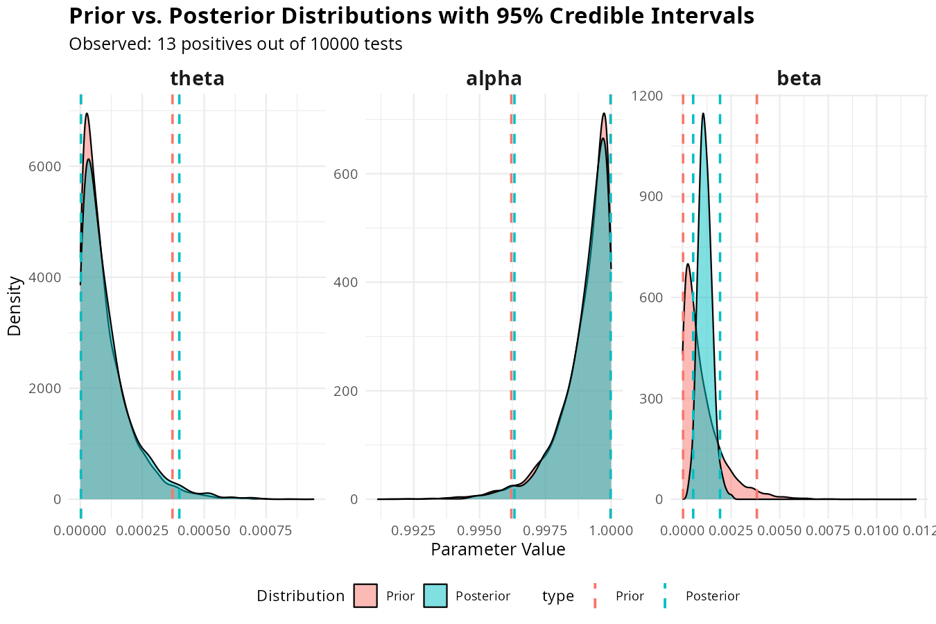
The output isn’t a single number — it’s a full joint posterior distribution over all three parameters. From this distribution, we can compute:
- The mean (our best point estimate) for each parameter.
- The median (another point estimate).
- Credible intervals (e.g., “there’s a 95% chance the true prevalence is between 0.008% and 0.012%”).
- The full shape of uncertainty for each parameter.
- Derived quantities like the Positive Predictive Value (PPV).

---

The Posterior Predictive Distribution

For a new individual with a positive test result, the probability they are actually sick is the Positive Predictive Value (PPV). That is the probability of being true positive over the probability of being positive:

\[ \text{PPV}(\theta, \alpha, \beta) = \frac{\alpha \cdot \theta}{\alpha \cdot \theta + \beta \cdot (1 - \theta)} \]

Since we don’t know the true values of \(\theta\), \(\alpha\), and \(\beta\), we need to account for our uncertainty about them.

PPV (\(P(\text{Sick}|\text{Positive})\)) is a standard, widely used concept in biostatistics, epidemiology, and clinical diagnostics, together with its complement, the Negative Predictive Value (NPV, \(P(\text{No Sick}|\text{Negative})\)).

The Posterior Mean (Point Estimate) If we want a single best estimate of the PPV, we compute its expected value under the posterior distribution:

\[ \mathbb{E}[\text{PPV} | \text{Positive}] = \int_0^1 \int_0^1 \int_0^1 \frac{\alpha \cdot \theta}{\alpha \cdot \theta + \beta \cdot (1 - \theta)} \cdot P(\theta, \alpha, \beta | \text{Positive}) \, d\theta \, d\alpha \, d\beta \]

This triple integral gives us a single number — the expected PPV, averaged over all parameter values weighted by their posterior probability. This is our best point estimate for the probability that a new positive-tested individual is actually sick.

The Full Posterior Predictive Distribution

1. Sampling from the joint posterior: draw many samples of \((\theta, \alpha, \beta)\) from \(P(\theta, \alpha, \beta | \text{Positive})\).
   
2. For each sample, compute the PPV:
   \[ \text{PPV}^{(i)} = \frac{\alpha^{(i)} \cdot \theta^{(i)}}{\alpha^{(i)} \cdot \theta^{(i)} + \beta^{(i)} \cdot (1 - \theta^{(i)})} \]
   
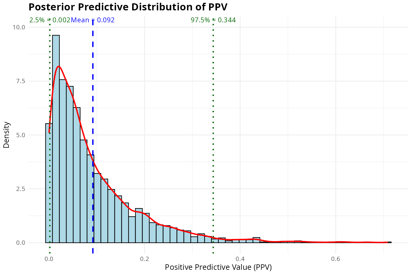
3. The collection of \(\text{PPV}^{(i)}\) values forms a one-dimensional distribution of PPVs — capturing our uncertainty about the true PPV.

This is the power of full Bayesian inference: we get distributions over everything, not just point estimates.

---

The Stan Model

Here is the complete Stan code implementing this full Bayesian model:

// Full Bayesian Model for Disease Testing
// Observed data: total positive tests only (individual sick status unknown)
data {
  int<lower=0> N;           // Total number of people tested
  int<lower=0> Positive;    // Total number of positive test results
}
parameters {
  real<lower=0, upper=1> theta;    // Prevalence: P(Sick)
  real<lower=0, upper=1> alpha;    // Sensitivity: P(Positive | Sick)
  real<lower=0, upper=1> beta;     // False Positive Rate: P(Positive | No Sick)
}
transformed parameters {
  real<lower=0, upper=1> p_positive;   // Overall probability of a positive test
  p_positive = alpha * theta + beta * (1 - theta);
}
model {
  // Priors
  theta ~ beta(1, 9999);      // Prevalence around 0.01%
  alpha ~ beta(999, 1);       // Sensitivity around 99.9%
  beta ~ beta(1, 999);        // False positive rate around 0.1%
  
  // Likelihood
  Positive ~ binomial(N, p_positive);
}
generated quantities {
  // Positive Predictive Value (PPV)
  // Probability of actually being sick given a positive test
  real PPV = (alpha * theta) / (alpha * theta + beta * (1 - theta));
  // Simulated positive count from the posterior predictive distribution
  int pred_Positive = binomial_rng(N, p_positive);
}

Unfold to see the R code running this inference

#### Simulate Data ####
# Simulate data (in real application, use actual observed data)
set.seed(42)
N <- 10000
true_theta <- 0.0001
true_alpha <- 0.999
true_beta <- 0.001

# Generate individual-level data
sick_status <- rbinom(N, 1, true_theta)
test_result <- ifelse(
  sick_status == 1,
  rbinom(N, 1, true_alpha),
  rbinom(N, 1, true_beta)
)

# Observed data (we only observe these!)
Positive <- sum(test_result)
N_observed <- N

# Prepare data for Stan
stan_data <- list(
  N = N_observed,
  Positive = Positive
)

#### Fit the model using Stan ####
# Fit the model
fit <- stan(
  file = paste0(current_dir, "/rare_disease.stan"),
  data = stan_data,
  chains = 4,
  iter = 2000,
  warmup = 1000
)

# Print summary
print(fit, pars = c("theta", "alpha", "beta", "PPV"))

# Plot posterior distributions
stan_dens(fit, pars = c("theta", "alpha", "beta", "PPV"))

# Extract posterior samples
posterior_samples <- rstan::extract(fit)

For how to assess convergence and model fit, see the tumour-growth-state-space model post.

---

What This Model Gives You

Running this model produces:

• Posterior distributions and Credible intervals for \(\theta\), \(\alpha\), and \(\beta\) — not just point estimates.
  

• Posterior predictive distribution for PPV — the probability of being sick given a positive test, fully accounting for uncertainty in all three parameters.
  

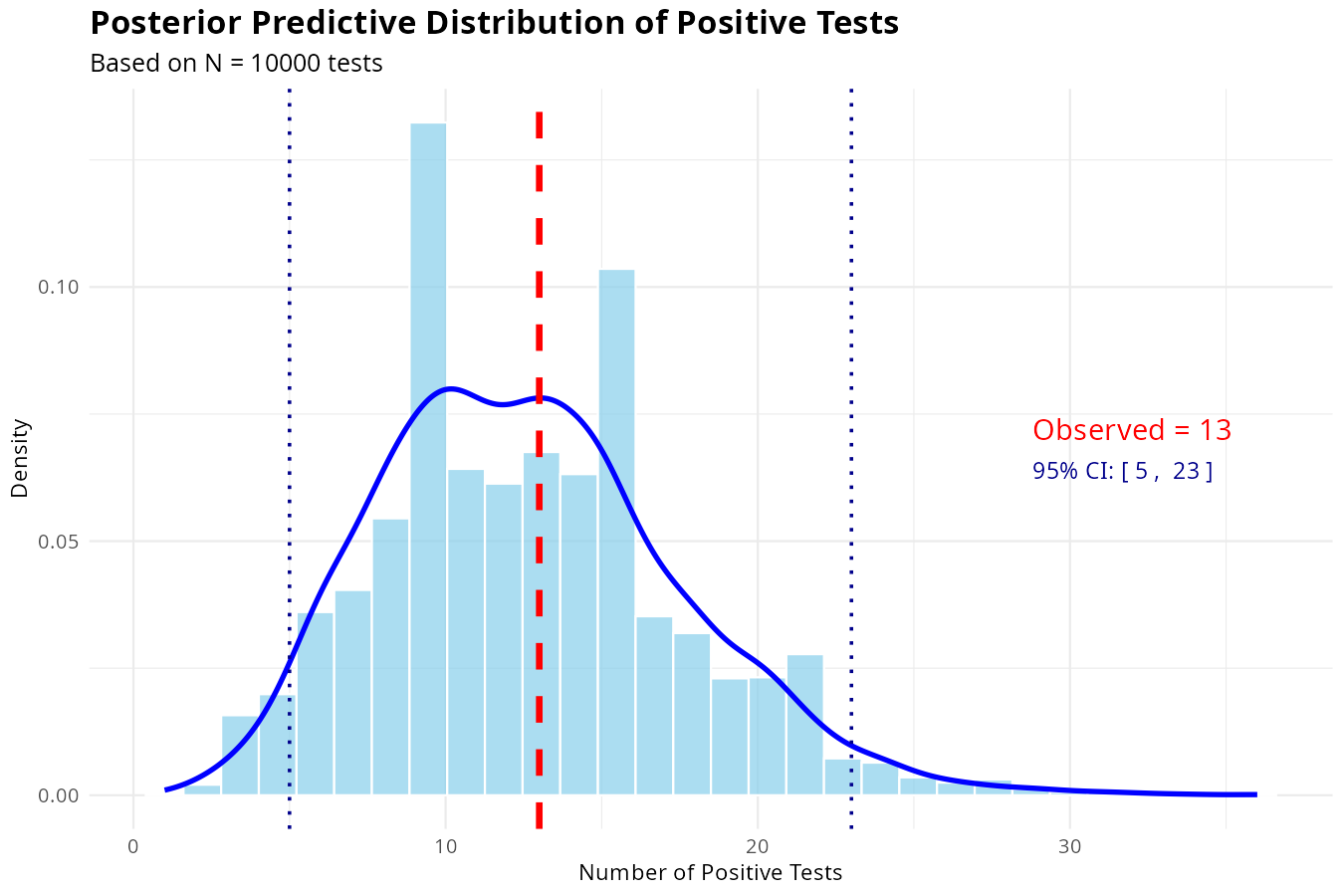
• Posterior predictive distribution for positives given N number of tests — simulated data from the model to compare against observed data.

---

Final Thoughts on Priors and the Danger of Unfalsifiable Beliefs

The prior is where Bayesian statistics gets interesting — and where it gets criticized. Opponents say priors are subjective. “You’re just making stuff up!” they cry.

But here’s the thing: priors are also the superpower of Bayesian thinking. They allow us to bring background knowledge, past experience, and expert judgment into the analysis. In this rare disease example, without priors, we will not be able to know the few positive test count is due to the low disease prevelence or inaccuracy of the screening. Therefore, prior knowledge makes these parameters identifiable.

Great power comes with great responsibility. If your prior is too strong, it can overwhelm the data and lead to misleading conclusions. If it’s too weak, it can fail to incorporate valuable knowledge. Best prior is always based on actual prior data and prior knowledge. Prior is also a quantitative way to record your experience, as well as constraints.

Here’s where Bayesian thinking becomes a life philosophy, not just a statistical tool.

Every belief should be falsifiable — it should be possible, in principle, to prove it wrong.

Why? Because if your prior assigns probability 1 to a hypothesis — no amount of data can disprove it, no Bayesian updating will shift the prior beliefs over time, and no evidence will ever change your mind — that’s not science, it’s dogma.

These are my principles for defining a prior (as well as for life in general!):

• Be explicit about what you believe before seeing data.
• Be humble — your beliefs should be open to revision.
• Be honest — if your belief can’t be disproven, it’s not a scientific belief. And if you know nothing about the data and associated parameters, maybe you should not conduct any test.