Mapping the Landscape of Chance – Distributions & A Glimpse of Bayes
Random Variables and Probability Distribution
When we measure something—someone’s blood pressure, today’s rainfall, the number of clicks on an ad—we rarely believe that number fell from the sky fully formed. Instead, we model it as a single draw from an underlying random process. Formally, we say the observed value \(y\) is a realisation of a random variable \(Y\), whose behaviour is governed by parameters \(\theta\). The parameters represent the latent truth we care about: the true mean blood pressure in a population, the true click-through rate of a campaign, the true bias of a coin. The data \(y\) is then a noisy measurement of that hidden reality, perturbed by natural variability. This is a profound shift in thinking: we move from treating data as fixed facts to seeing data as signals that carry information about deeper, unobserved truths.
Once we’ve framed data as draws from a random variable \(Y\), we need a way to describe \(Y\)’s full behaviour. That’s the probability distribution. It’s a precise mathematical function that assigns a number to every possible outcome the random variable can produce.
For discrete outcomes (countable things like the number of heads, the number of emails received), we use a Probability Mass Function (PMF): it gives the probability \(P(Y = k)\) for each specific value \(k\). For continuous outcomes (measurements like height, temperature, waiting time that are on a smooth scale), we use a Probability Density Function (PDF): the density \(f(y)\) at a single point isn’t a probability by itself, but the area under the curve over an interval gives \(P(a < Y < b)\). Either way, the distribution is the full description of the random variable’s behaviour—telling you which values are likely, which are rare, and which are impossible. And parameters \(\theta\) control its centre, spread and shape. A probability distribution must obey Rule No. 4: the sum (or integral) of all probabilities across the entire sample space is exactly 1.
Example A survey finds that 18% of households have no children, 25% have one, 35% have two, 15% have three, 5% have four, and 2% have five or more. These probabilities sum to 1, and together they form the PMF of the discrete random variable \(Y =\) “number of children.” This distribution lets you answer questions like “What’s the chance a randomly chosen household has at least two children?” without surveying the entire country again.
Common discrete distributions and their real-world fingerprints:
- Binomial: Number of successes in a fixed number of trials (e.g., how many of 20 job applicants pass an interview).
- Poisson: Number of events in a fixed interval (e.g., number of earthquakes per year in a region, number of calls to a helpline per minute).
- Geometric: Number of trials until the first success (e.g., how many Tinder swipes until a match).
Common continuous distributions:
- Normal (Gaussian): The classic bell curve—heights, blood pressure, measurement errors.
- Exponential: Waiting times between events (e.g., time until the next earthquake, time until a lightbulb burns out).
- Uniform: Every outcome in an interval is equally likely (e.g., a randomly chosen number between 0 and 1).
A Closer Look: The Binomial Distribution
When we assume our variable \(Y\) follows a particular named distribution, we use the tilde notation: \[Y \sim \text{Binomial}(n, p)\]
The Binomial distribution is the workhorse for counting successes in a fixed number of independent trials, each with the same success probability. Think: flip a biased coin \(n\) times, count the heads. The parameters are: - \(n\): number of trials (how many flips, how many applicants, how many patients). - \(p\): probability of success on each trial (how biased the coin, how hard the interview, how effective the drug).
The distribution then answers: “What’s the probability of getting exactly \(k\) successes?” It’s a discrete distribution, so it has a PMF, and the possible outcomes range from 0 to \(n\). If the probability of getting a head in each toss, \(p\), is 0.2 (a biased coin), the distribution would skew towards low head counts, as shown below.
# Simulate 10,000 experiments of 10 fair coin flips each
n_flips <- 10
prob_heads <- 0.2
n_sims <- 10000
simulated_heads <- rbinom(n_sims, size = n_flips, prob = prob_heads)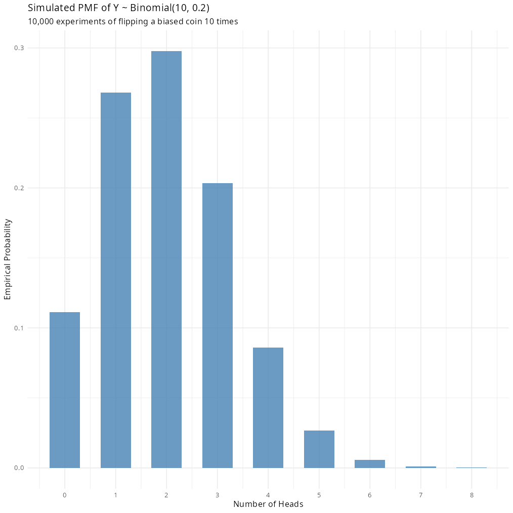
A Whisper of Bayes: Turning the Arrow
Everything we’ve done so far treats parameters \(\theta\) (the \(n\) and \(p\) in our Binomial, or the population mean and standard deviation in our Normal) as a fixed, unknown truth. We ask: “Given these fixed parameters, how likely is the data we see?” That’s \(p(y|\theta)\).
Bayesian statistics dares to ask a different question: “Why should data be the only uncertain thing?” What if we’re also uncertain about the parameters themselves? It treats \(\theta\) not as fixed points but as variables with their own probability distributions. This is the prior distributions, \(p(\theta)\), capturing our belief before seeing the current data.
The engine then hums to life. The familiar \(p(y|\theta)\) is now the likelihood, the story the data tells about the parameter. Through Bayes’ theorem, these two are combined to form the posterior distributions: \[p(\theta|y) \propto p(y|\theta) \cdot p(\theta)\] The arrow of inference turns from \(p(y|\theta)\) (data given parameter) to \(p(\theta|y)\) (parameter given data). The parameter transforms from a single number into a whole landscape of plausible values, updated by evidence. That’s where we’re headed next.