The Mind’s Guide to Chance – The Rules of the Game
The chance of you using probability to navigate life is remarkably high. You glance at a weather forecast and silently calculate the odds before choosing an outfit. You weigh the likelihood of success before hitting “submit” on a job application. You are, whether you realise it or not, already fluent in the language of chance.
And the chance of you being mapped into someone’s predictive matrix? Higher still. Netflix doesn’t just recommend shows—it calculates the probability you’ll binge a new series based on millions of viewing patterns like yours. Your insurance premium isn’t pulled from thin air; it’s a number derived from the estimated likelihood of you filing a claim, given your age, postcode, and driving history. Even the criminal justice system now uses algorithms that estimate the probability of re-offending to inform bail and sentencing decisions. Quietly, often invisibly, your life is being shaped by someone else’s models.
So understanding probability isn’t a mathematical luxury. It’s essential literacy for understanding the world—and for glimpsing how the world understands you.
Probability is not just numbers; it’s the formal language of uncertainty, a natural extension of logic’s rigid “true or false” into the nuanced world of “maybe”. Probability captures how strongly we believe an event will happen, anchoring our belief on a scale that, by its first and most fundamental rule, never strays below 0 or beyond 1.
Rule No. 1: For any event \(A\), its probability \(P(A)\) satisfies: \[0 \leq P(A) \leq 1\]
A simple way to feel this is the classic six-sided die. The probability of rolling a six isn’t just an abstract idea; it’s the long-run proportion of successes. If you roll the die 100 times and count how many times a six appears, you’re building an empirical bridge to the theoretical probability of \(\frac{1}{6}\).
Speaking in Odds: The Gambler’s Accent
Sometimes, belief is voiced not in probabilities but in odds. Walk into a betting shop, and you’ll hear this dialect. Crucially, odds are not the Odds Ratio, a separate tool we use to measure association between two events.
Odds are a ratio of hope to fear: the number of ways to succeed divided by the number of ways to fail. However, how to obtain odds depends on language: “4-to-1 odds against winning” means 4 chances of losing for every 1 chance of winning, resulting in odds of 1/4; whereas “4-to-1 in favour” means the opposite. Probability, on the other hand, is more precise. If the probability of an event \(A\) is \(P(A)\), the odds in its favour are calculated as a seesaw: \[\text{Odds}(A) = \frac{P(A)}{1 - P(A)}\] From this, we can effortlessly reconstruct the probability from the odds, moving from the gambler’s lingo back to our calibrated scale: \[P(A) = \frac{\text{Odds}(A)}{1 + \text{Odds}(A)}\] Example: If a bookie offers 4-to-1 odds against a long-shot horse, the implied probability of it winning is \(P(\text{Win}) = \frac{1/4}{1 + 1/4} = \frac{1}{5} = 0.2\). A 20% chance, not 25% as is often mistakenly thought.
The Art of Combination: AND
Life is rarely about a single event. It’s a web of coincidences and a chain of happenings. Sometimes events overlap by chance; sometimes they unfold step by step. The AND rule handles both patterns with the same elegant logic. We often need to know the chance that event \(A\) AND event \(B\) both occur. The foundational formula for this joint probability is: \[P(A \cap B) = P(A) \cdot P(B|A) = P(B) \cdot P(A|B)\] This reveals a deep truth: we’re multiplying the probability of one event by the probability of the other, given the first has occurred.
A special, powerful case emerges when events are independent—when one happening doesn’t whisper any secrets about the other. We get our Rule No. 2: Events \(A\) and \(B\) are independent if and only if: \[P(A \cap B) = P(A)P(B)\] Example: Rolling a die and flipping a coin. The \(P(\text{Roll a 4} \cap \text{Flip Heads})\) is simply \(\frac{1}{6} \cdot \frac{1}{2} = \frac{1}{12}\). The die doesn’t conspire with the coin.
Example: Drawing two cards from a standard deck of 52 cards, without putting the first one back. The probability that both are Aces is: \(P(\text{First Ace} \cap \text{Second Ace}) = P(\text{First Ace}) \cdot P(\text{Second Ace} \mid \text{First is Ace}) = \frac{4}{52} \cdot \frac{3}{51} \approx 0.0045\)
What about when we’re combining more than two events? The logic gracefully extends: \[P(A_{1} \cap A_{2} \cap ... \cap A_{n}) = P(A_{1}) \cdot P(A_{2}|A_{1}) \cdot ... \cdot P(A_{n}|A_{1} \cap ... \cap A_{n-1})\]
The Great Weighting: The Law of Total Probability
Imagine event \(B\) is a destination, and it can be reached through a set of distinct, non-overlapping paths—the “disjoint” events \(A_1, A_2, ..., A_n\) that carve up the entire sample space. The probability of arriving at \(B\) is simply the sum of the probabilities of traveling through each path, each weighted by how likely that path itself was: \[P(B) = \sum_{i=1}^{n} P(B \cap A_i) = \sum_{i=1}^{n} P(B|A_i)P(A_i)\] This is a remarkably powerful tool for breaking a complex probability into manageable pieces.
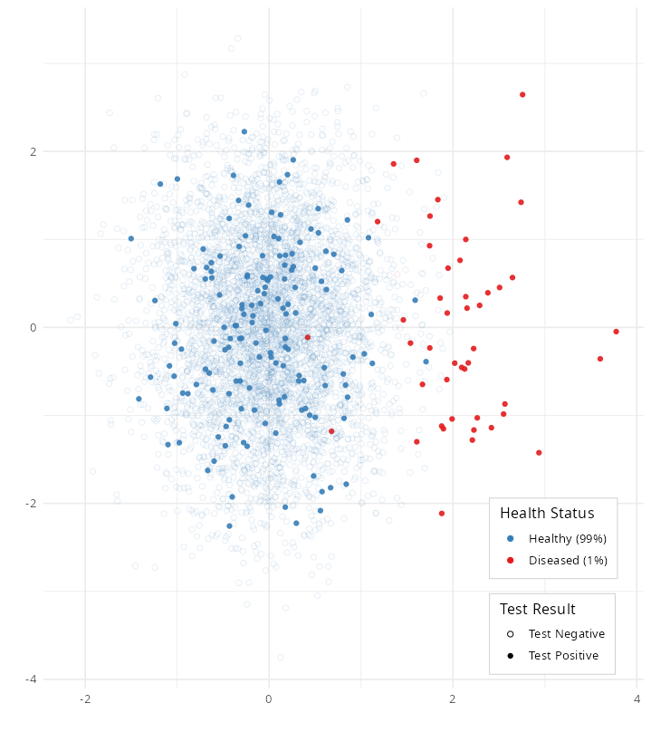
Example: Suppose a disease affects 1% of the population. A new test is 95% accurate on those who have the disease, but also returns a false positive 3% of the time on healthy people. What’s the overall probability someone tests positive?
Let \(D\) = has the disease, \(H\) = healthy. We know \(P(D) = 0.01\), \(P(H) = 0.99\), \(P(+|D) = 0.95\), and \(P(+|H) = 0.03\). The Law of Total Probability gives us \(P(+) = P(+|D) \cdot P(D) + P(+|H) \cdot P(H) = (0.95 \cdot 0.01) + (0.03 \cdot 0.99) = 0.0095 + 0.0297 = 0.0392\). About 3.9% of those tested get a positive result—far higher than the 1% disease rate, because the small false positive rate applies to the vast healthy majority. The law weights each path correctly: a tiny chance of catching a true positive, a much larger chance of a false alarm, combined into one answer.
The Art of Combination: OR
What about the chance that at least one of two events occurs? That’s the OR rule, our Rule No. 3: \[P(A \cup B) = P(A) + P(B) - P(A \cap B)\] We subtract the overlap because we’d otherwise be double-counting the region where both \(A\) and \(B\) are true. If the events are mutually exclusive (disjoint, no overlap), that last term vanishes, and the probability of one or the other is simply the sum of their individual probabilities. The chance of rolling a 1 or a 2 on a die is cleanly \(\frac{1}{6} + \frac{1}{6} = \frac{1}{3}\). However, the chance of rollwing a number less than 4 or greater than 2 is \(P(\text{<4} \cup \text{>2}) = P(\text{1,2,3}) + P(\text{3,4,5,6}) - P(\text{3}) = \frac{3}{6} + \frac{4}{6} - \frac{1}{6} = 1\).